
From Pythagoras to Fourier and From Geometry to Nature
DOI: https://doi.org/10.55060/b.p2fg2n.ch013.220215.016
Chapter 13. From Universal Natural Shapes to Scientific Methodology
13.1 Universal Natural Shapes
In Part I it was shown that Pythagoras’ theorem, linked to the concept of orthogonality of vectors, has received numerous extensions in modern mathematics, particularly in Hilbert spaces. Jean-Baptiste Joseph Fourier is certainly one of the most cited scholars on the applications of mathematics in technical literature. In fact, the introduction of the series and the transform that bear his name have allowed us to mathematically describe the most diverse physical phenomena, ranging from the theory of heat to that of vibrations and electromagnetic phenomena. Fourier series and transforms are indeed used in every corner of science and technology [70]. An implicit assumption underlying the Pythagorean theorem, its generalization for any triangle, Fourier series and Hilbert spaces, is that spaces are somehow isotropic, i.e. the same in all directions. The locus of points that one arrives at after a prescribed period of time starting from one point and going in any direction will result in the classic Euclidean circle as unit circle. But in nature circles are not common and precisely the reason why Gabriel Lamé made the connection between his curves and crystals.
A.C. Thompson: “Space to Euclid and Newton was uniform and “isotropic”, the same in all directions. Such a notion flies in the face of daily experience, where the connotation of up and down is different from that of east to west. There are preferred directions. Another good example is the preferred directions that cause crystals to grow as polyhedra and not spherically like soap bubbles. Unit circles and spheres are not the familiar round objects from Euclidean geometry, but are some other convex shape, called the unit ball.” [99]
The geometer Leopold Verstraelen wrote: “In the same way as Euclidean geometry in dimension 2 essentially derives from the circle as ground figure by which distances may be determined in an isotropic way when considered from a human point of view, the Lamé curves are at the basis of the simplest definite Minkowski-Finsler geometries in which 4-fold anisotropies occur when considered from a human point of view, and analogous observations can be made in dimensions 3 and more. In this respect, the so-called Gielis curves for dimension 2 and Gielis (hyper)surfaces for dimension 3 (and more) turned out to be ground figures for describing most natural s-fold anisotropies (for s = 0, 1, 2, 3, 4, 5, … , or, for that matter, for any s ∈ R). And, closely related herewith, by application of the corresponding Gielis transformations to the “most natural” curves and surfaces of Euclidean geometry (e.g. for dimension 2: the circles amongst the closed curves and the logarithmic spirals amongst the non-closed curves), do result many of the forms that we do observe in nature – in biology, crystallography, physics, chemistry, etc.” [102]
These transformations give rise to the simplest Riemann-Finsler geometries (Section 9.1). At the same time, they are a generalization of the Pythagorean theorem making use of the classic trigonometric functions and the four principal mathematical operations. The question whether Fourier techniques could be used on such anisotropic domains has been answered affirmatively in Part III, also for the original problem of Fourier, but now on a starlike domain [73]. The focus in Part III was on Gielis domains, but the method of the stretched Laplacian is very general. It should also be noted that convergence is very fast, typically less than 10 steps to minimize error. This is of great importance for the natural sciences because existing mathematical techniques can be used (Part III). Describing the Laplacian for a stretchable radius, separation of variables can be used and Fourier-projection methods led to a solution of boundary value problems (Laplace, Helmholtz and Poisson equations) on all normal polar 2D and 3D domains, including Riemann surfaces, for various boundary conditions.
This stands in stark contrast to how technology developed. Fourier’s original method could be used on a circular domain (“heat plate”). A few other methods like conformal mapping allowed for extending these domains, but the statement that finite elements were developed to address this problem of limited domains is not far from the truth. The situation was summarized by Richard Feynman [34]: “The mathematical problem of the direct method is the solution of Laplace’s equation Δ2φ = 0. Subject to the condition that φ is a suitable constant on certain boundaries – the surfaces of the conductors. Problems which involve the solution of differential field equations subject to certain boundary conditions are called boundary value problems. They have been the subject of considerable mathematical study. In the case of conductors having complicated shapes, there are no general analytical methods. Even such a simple problem as that of a charged cylindrical metal closed at both ends – a beer can – presents formidable mathematical difficulties. It can be solved only approximately, using numerical methods. The only general methods of solution are numerical.” Two centuries after Fourier, the availability of a continuous transform allows for exact solutions on a wide range of domains in 2D and 3D without the need for meshing. This can be achieved by generalizing the Laplacian and solving boundary value problems on any domain. The next step is to couple shapes and development of shapes to natural curvature conditions (Section 14.2).
13.2 A Wide Range of Natural and Abstract Shapes
The title of the original paper introducing Gielis transformations in the American Journal of Botany is “A Generic Geometric Transformation That Unifies a Wide Range of Natural and Abstract Shapes” [40]. ‘Generic’ points to the applicability of a wide group of shapes, forms and phenomena, but the term ‘Unifies’ specifies that this transformation not only works for the abstract shapes in mathematics, but also for natural shapes. In this section, a range of natural and abstract shapes described by this transformation are juxtaposed (Figures 43–47).
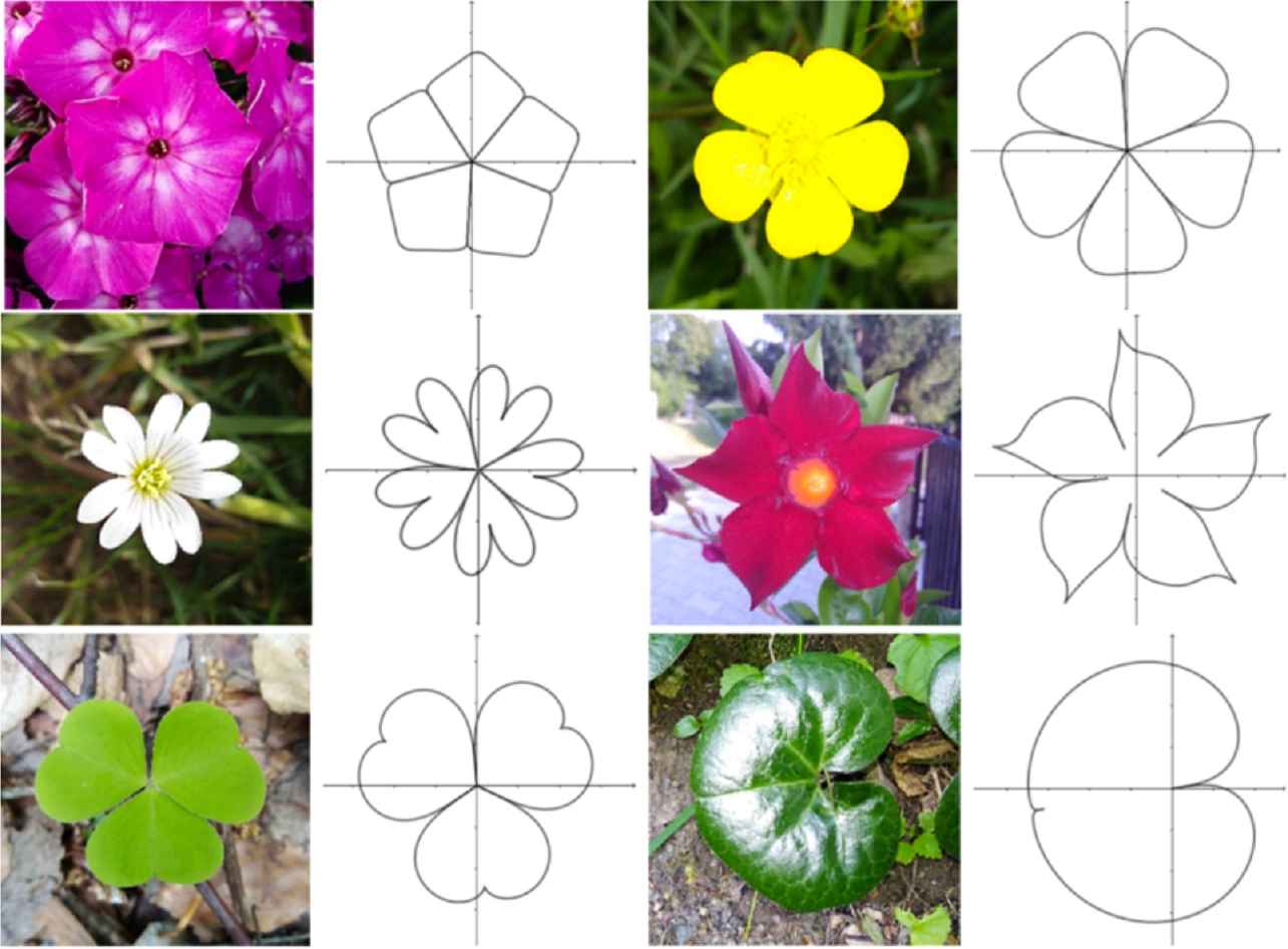
Advancing geometric description of plant organs.
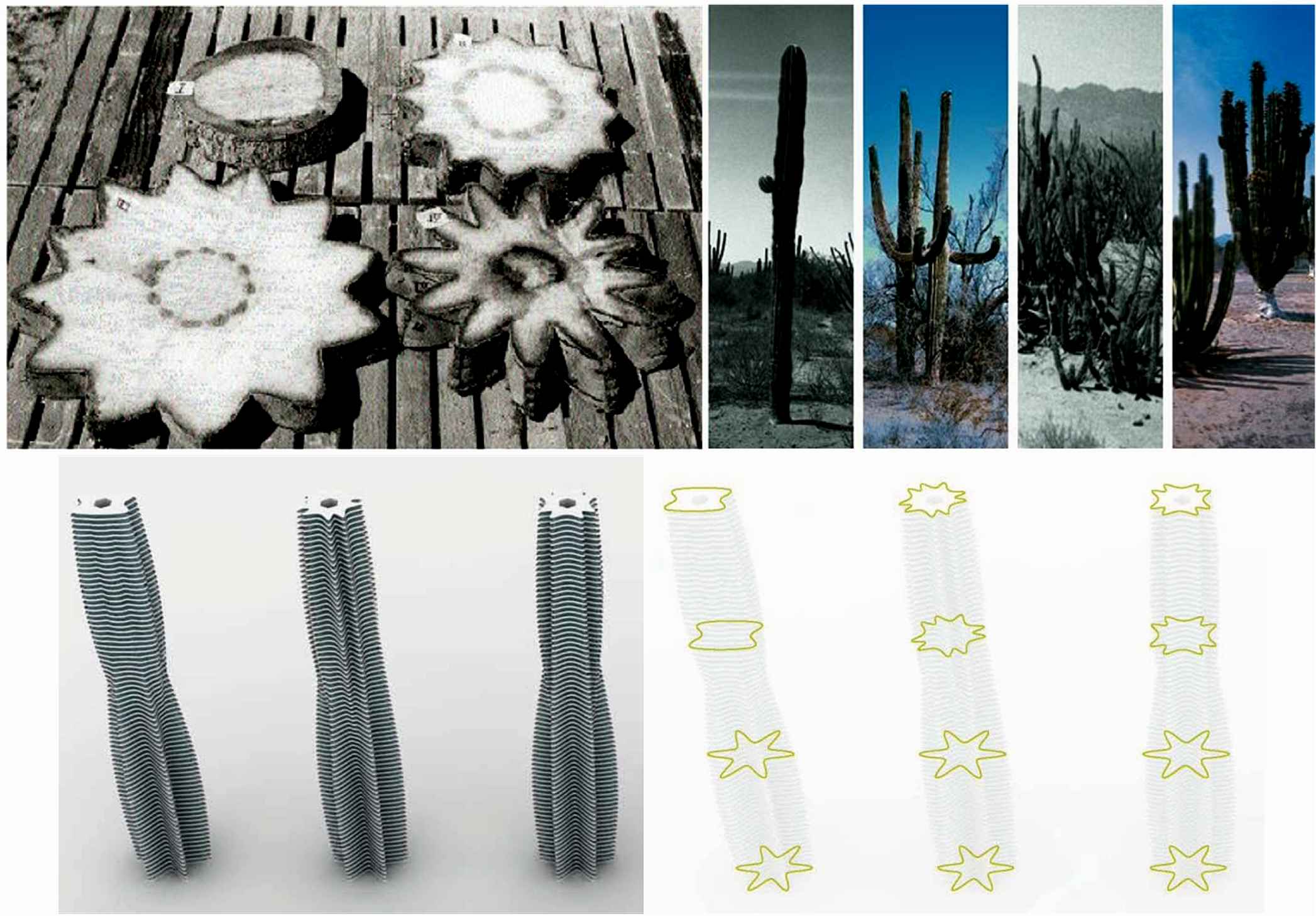
Top row: columnar cacti and sections [41]. Bottom row: Superformula Towers by Lava Architects and their sections in green.
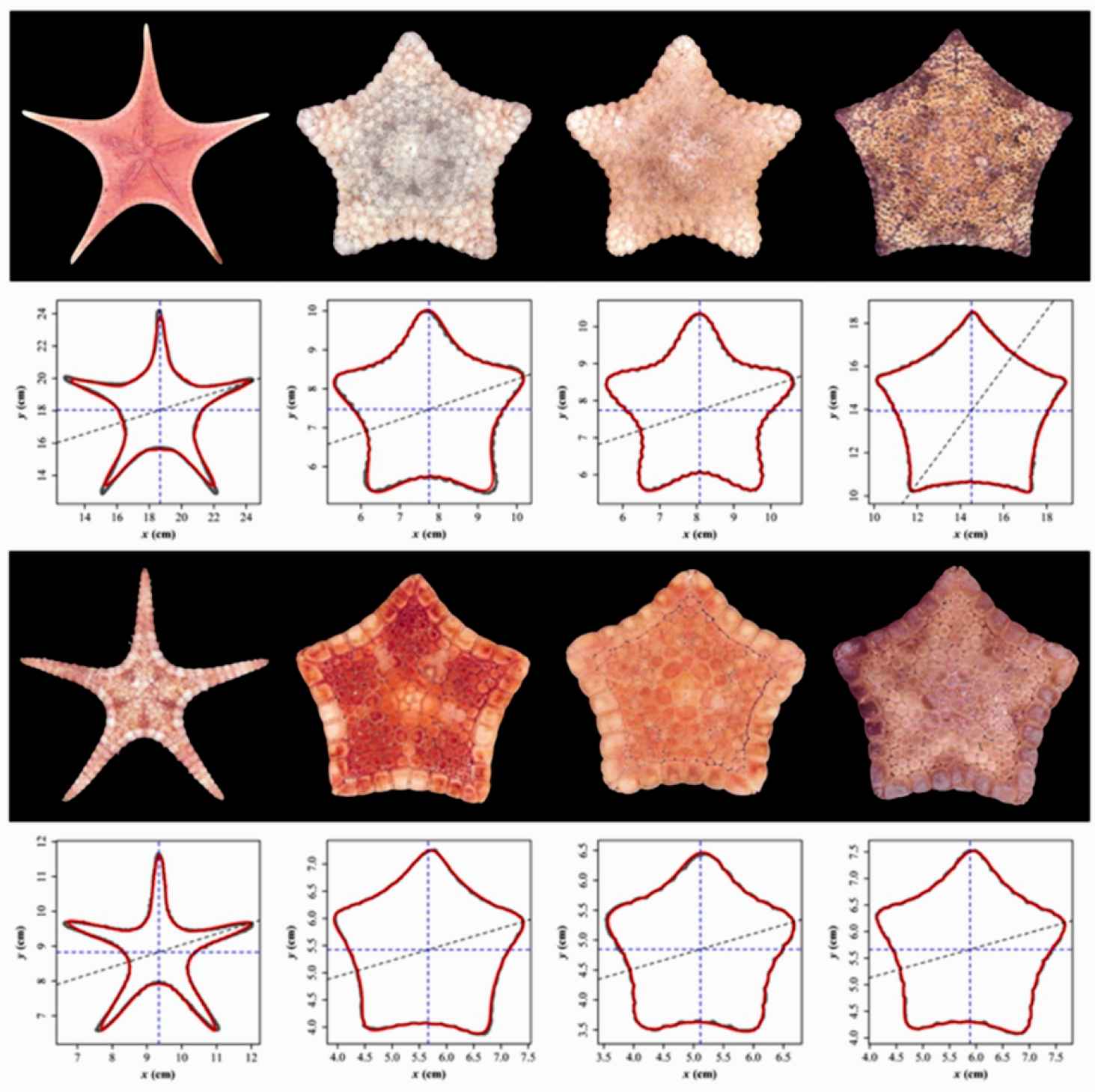
Upper left: Anthenoides tenuis. Upper row: Culcita schmideliana. Lower left: Stellaster equestris. Lower center left and lower center right: Tosia australis. Lower right: Tosia magnifica [88].
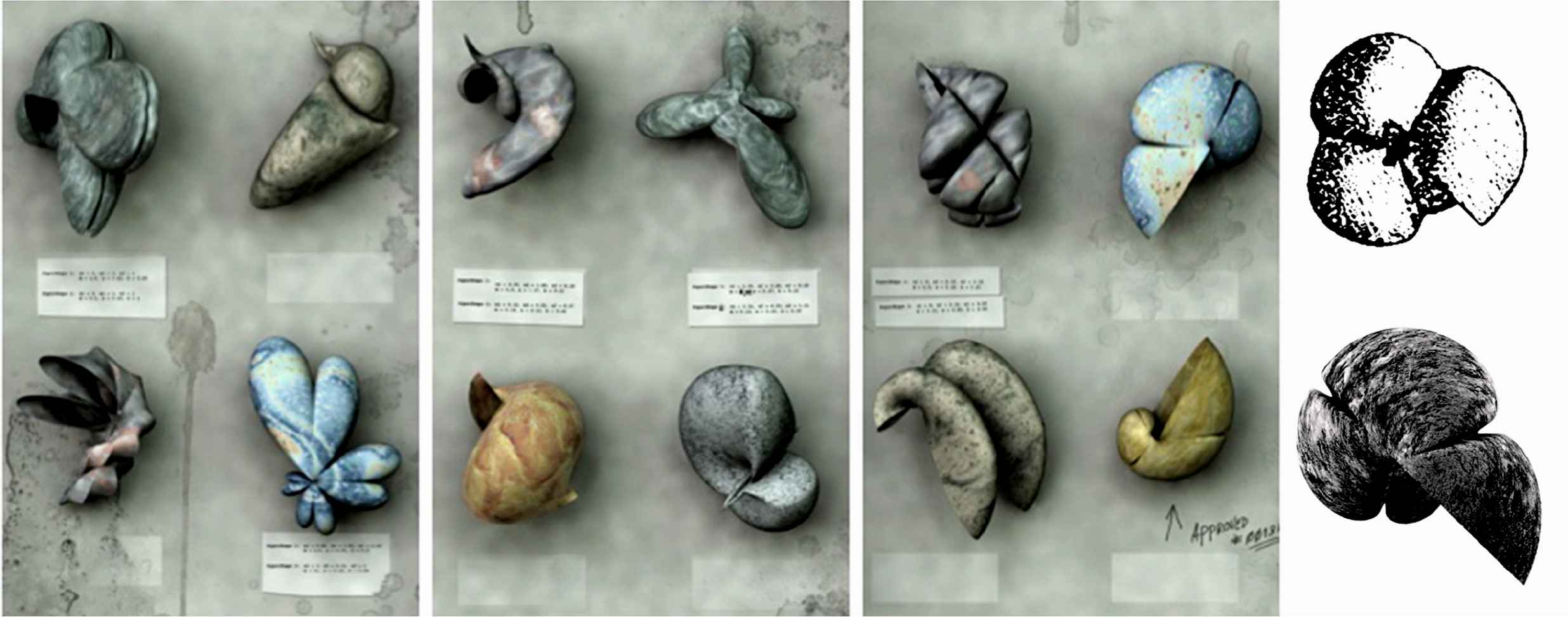
Future Fossils. Top right: fossil of a Parawocklumeria shell with constrictions. Bottom right: one of the Future Fossils with constrictions.
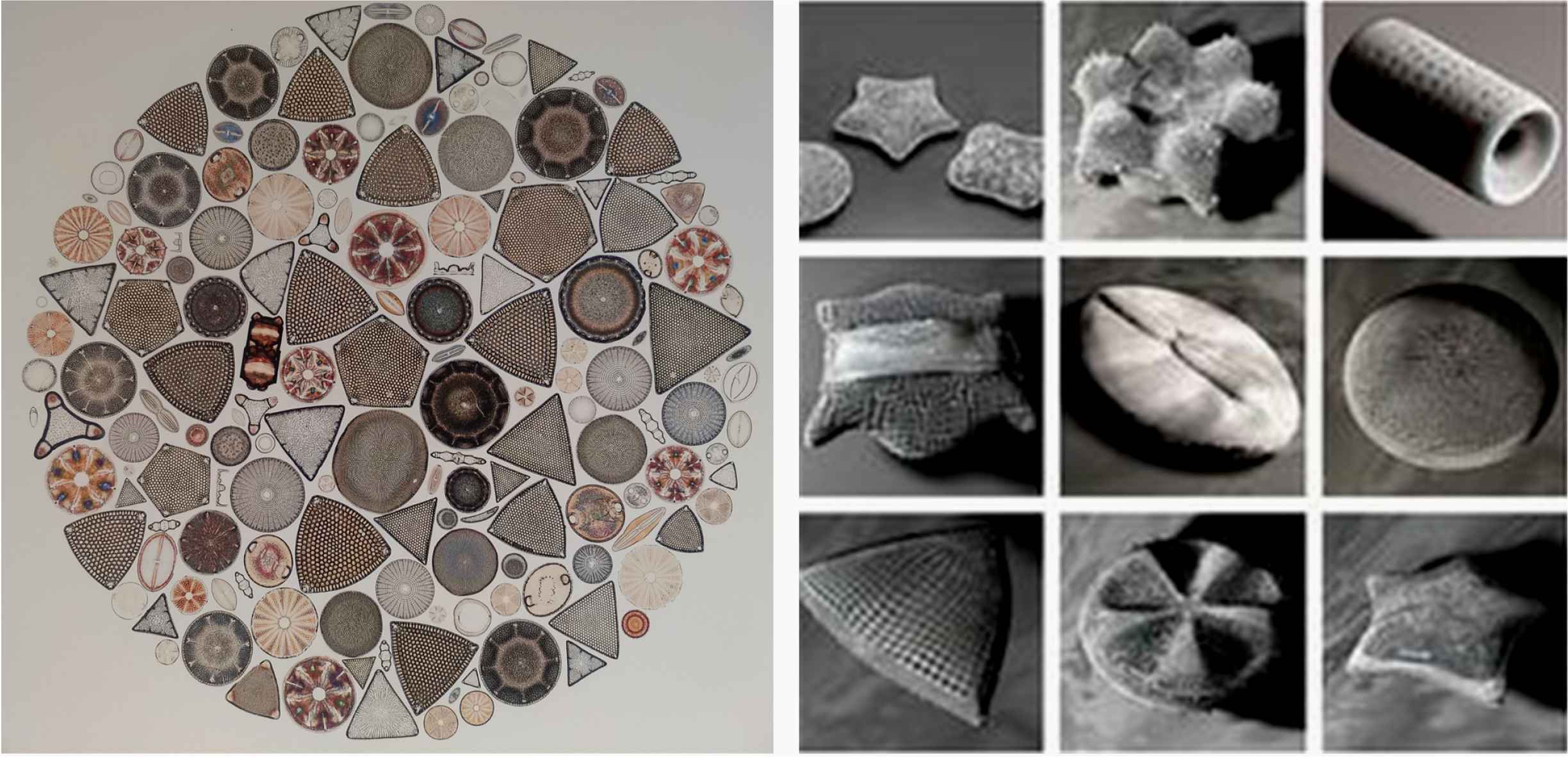
Left: Diatoms – biological. Right: Diatoms – digital (www.mrkism.com).
13.3 What Can We Do With Two (or Three) Parameters?
Superellipses are closed Lamé curves and they are widely used now even in astronomy (Figure 48; [26, 47, 94]). They have also been used in architecture worldwide. The most illustrious example is Sergel’s Torg in Stockholm. Piet Hein suggested to the architects to use a superellipse to optimize space and obtain a uniform curve (Figure 49), whereas the architects originally used various arcs [37, 41].
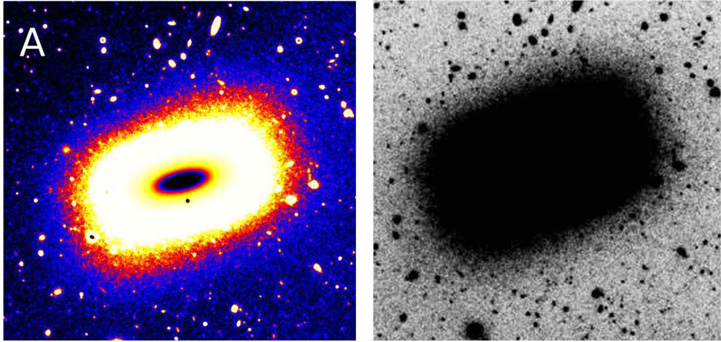
A superelliptical galaxy: LEDA 074886 [52].
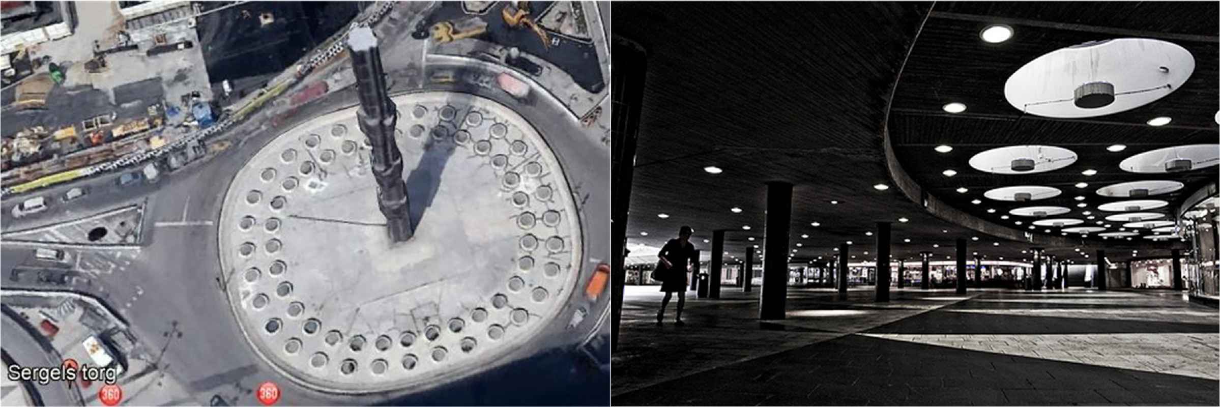
Sergel’s Torg in Stockholm.
This was the inspiration to describe the cross sections of square bamboos Chimonobambusa quadrangularis using superellipses in plants [40, 42]. This hypothesis was tested on more than 1,436 sections of another square bamboo, Chimonobambusa utilis (Keng) [59]. This is a medium to large bamboo with culms 5–10 m tall and 3–4 cm in diameter, characterized by quadrangular cross sections in the lower and middle parts of the culms.
This species of bamboo is distributed over a wide area in Sichuan, Guizhou and Yunnan provinces in China at altitudes of 1,400 to 2,600 m and average temperatures of 8–16°C, with extreme low temperatures of −14°C. The name ‘chimono’ derives from the Greek word for winter.
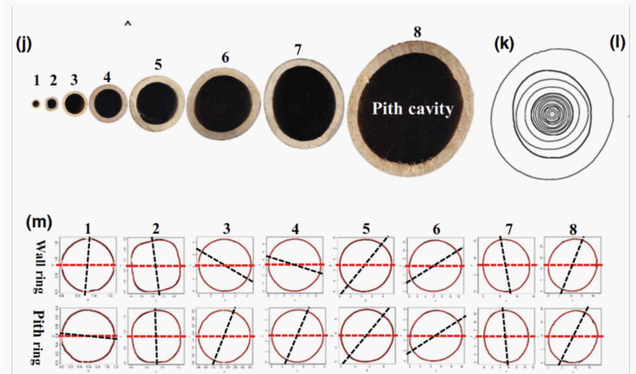
Indeed, the shoots of these species develop in autumn, typically from late August to December, in contrast to all other temperate bamboos with new shoots sprouting to full height in spring and with lignification throughout the season. The elongation of square bamboos can halt due to the cold and start again in spring to attain their full height. The particular cross-sectional shape of the culms is beneficial with improved resistance against torsion and bending [41]. From 30 stems, 750 sections were cut, leading to 1,436 shapes to be analyzed with the shape of the outer and inner rings (Figure 50). All tested bamboo culms can be described by superellipses (Figure 51).
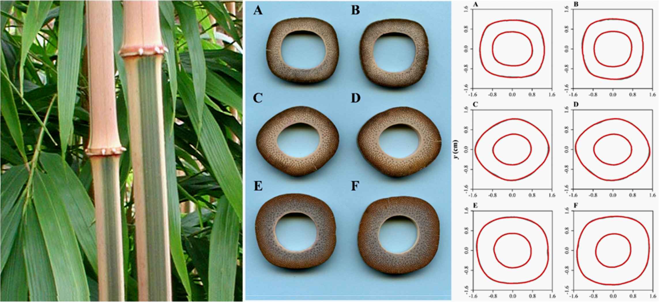
Left: culms of Chimonobambusa quadrangularis ‘Suow’. Center and right: cross sections of Chimonobambusa utilis and fitted curves.
Bamboo culms [104].
One crucial finding in square bamboo stems of Chimonobambusa utilis is a bimodal distribution of superellipses with n > 2 and subellipses with n < 2 in Figure 52A and 52B respectively [59]. In particular, and most pronounced in the outer rings, we find no ellipses (or circles) at all (Figure 52). We find only super- or subellipses (not deviations from ellipses). This effect is more outspoken in the outer rings, but one is reminded of the fact that the tissues furthest from the center contribute most to counteracting forces of bending and torsion.
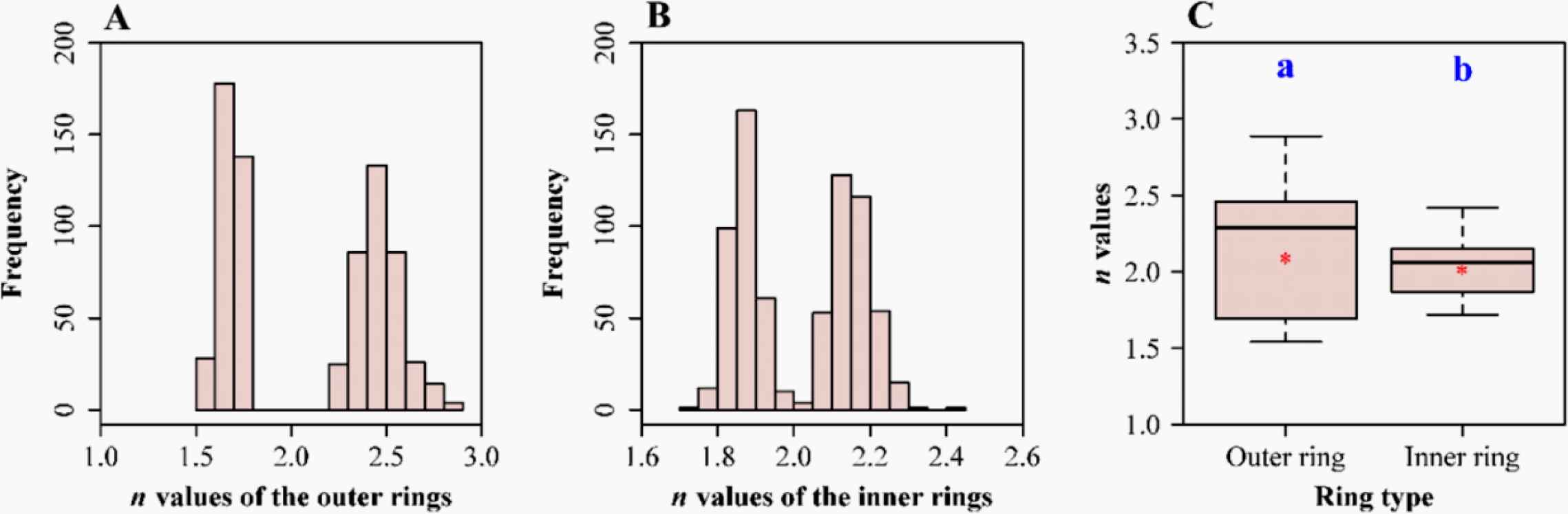
Bimodal distribution of n values of outer rings (A) and inner rings (B). The boxplot (C) shows mean and median as well as standard deviations.
The shape of cross sections of bamboo culms is described by two parameters, namely one for the shape (n) and one for the size (a/b):
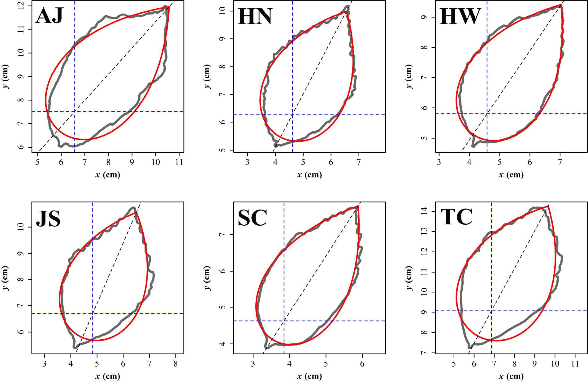
It turns out that for a wide range of natural shapes, a low-parameter version of GT is sufficient. For example, also the shape of bamboo leaves is encoded in two parameters, one for the shape n and one for the size, and the predicted leaf shape matched the observed leaf shape very well for 46 bamboo species (Figure 53). In this case, the relevant fitting is given by:
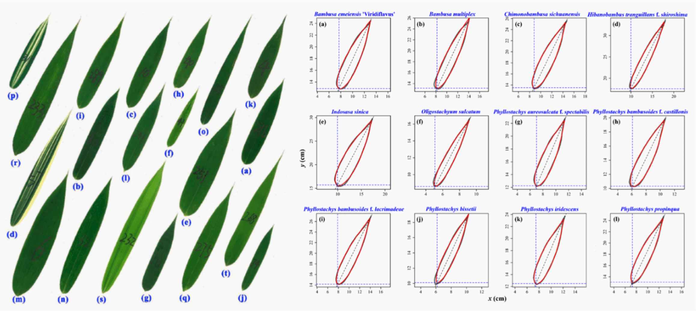
Left: leaves of various bamboos. Right: comparison between scanned leaf profile and predicted leaf profile [68].
Although the leaf sizes (length and width) of all 46 tested bamboo species differ considerably, their leaf shapes vary relatively little, but the difference can be clearly quantified [68]. Whereas in taxonomy bamboo leaf blades are characterized by qualitative characteristics such as lanceolate and linear-lanceolate, we now have a clear quantitative number (the exponent) for a qualitative characteristic. Only two parameters account for variations in shape and size between different bamboo species.
This can also be used for a wide variety of plant leaves (or leaflets on compound leaves). Figure 54 shows fits of superelliptical curves to leaves of Parrotia [89], where the area of the leaf and the fitted two-parameter curve are the same. Note that area, not shape, is the most important characteristic of foliage leaves in plants, aimed at maximizing the area available for photosynthesis.
Leaves of Parrotia [89].
Equation (13.1) was also used as a method to study the tree rings of seven different conifers or softwoods [87]. In general, cross sections of softwood trees suggest a circular shape for the tree rings, but perception can be very misleading. It was shown that tree rings are much better modeled by superellipses (Figure 55). The modified version of the Gielis formula used is with all exponents n equal and with a and b different, which starts from superellipses. Measuring hundreds of tree rings proved that the model was very efficient. In softwoods it is well known that the stems tend to spiral and may change direction after some time. This rotation around the vertical axis is torsion, relative to the axis as a cylinder, and it has both genetic and environmental components. The study of tree rings with Equation (13.1) permits a quantification of the rotation of tree rings over the years and is one of the very first in its kind to focus on this aspect of growth in trees.
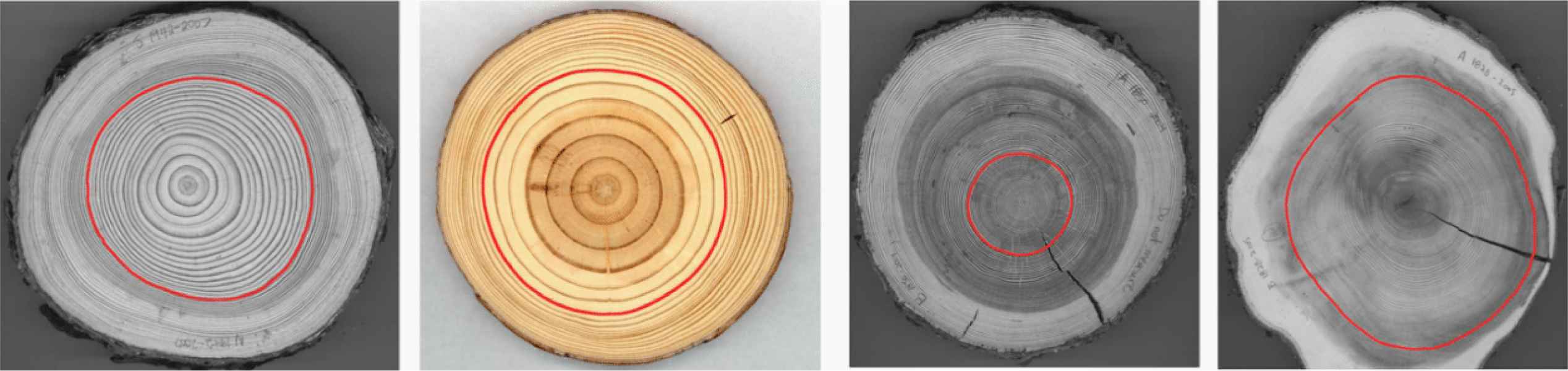
Superelliptical tree rings in softwoods. From left to right: Jack pine (Pinus banksiana Lamb), red pine (Pinus resinosa Aiton), tamarack (Larix laricina (Du Roi) K. Koch) and white cedar (Thuja occidentalis L.).
The model is also dynamic. The volume, size and shape of cross sections (area and perimeter) of cacti changes depending on how much water is stored in the cactus: it will expand after rainfall and shrink in drier periods. Having these characteristics available, immediately permits the study of such ratios in more depth. Ratios such as area/perimeter or area/polar moment of inertia, etc. can be used. Plants have to adapt continuously to changing environments caused by temperature, rainfall and wind, and have to perform multi-objective optimization. Superellipses and supershapes are excellent solutions [41].
13.4 Chebyshev for Botanists
Fibonacci numbers are a very popular subject of research and recreation, and one can find innumerable articles on the topic in mathematics, science, architecture and the arts. Especially in the latter fields they have achieved an almost divine status, because of the relation to the golden mean. From a scientific point of view however, one needs to be very cautious in the application of the series to actual natural or cultural phenomena. For example, in the arrangement of leaves, the Fibonacci numbers relate the number of spirals going in one direction to the number of spirals in the other (Figure 56). In a large-scale experiment of popular science with over 600 sunflowers, only 3 out of 4 of the parastichies on sunflowers were direct Fibonacci numbers. The other 1/4 (i.e. 25%) were approximate or modified Fibonacci and Lucas numbers, derived series, or irregular [95].
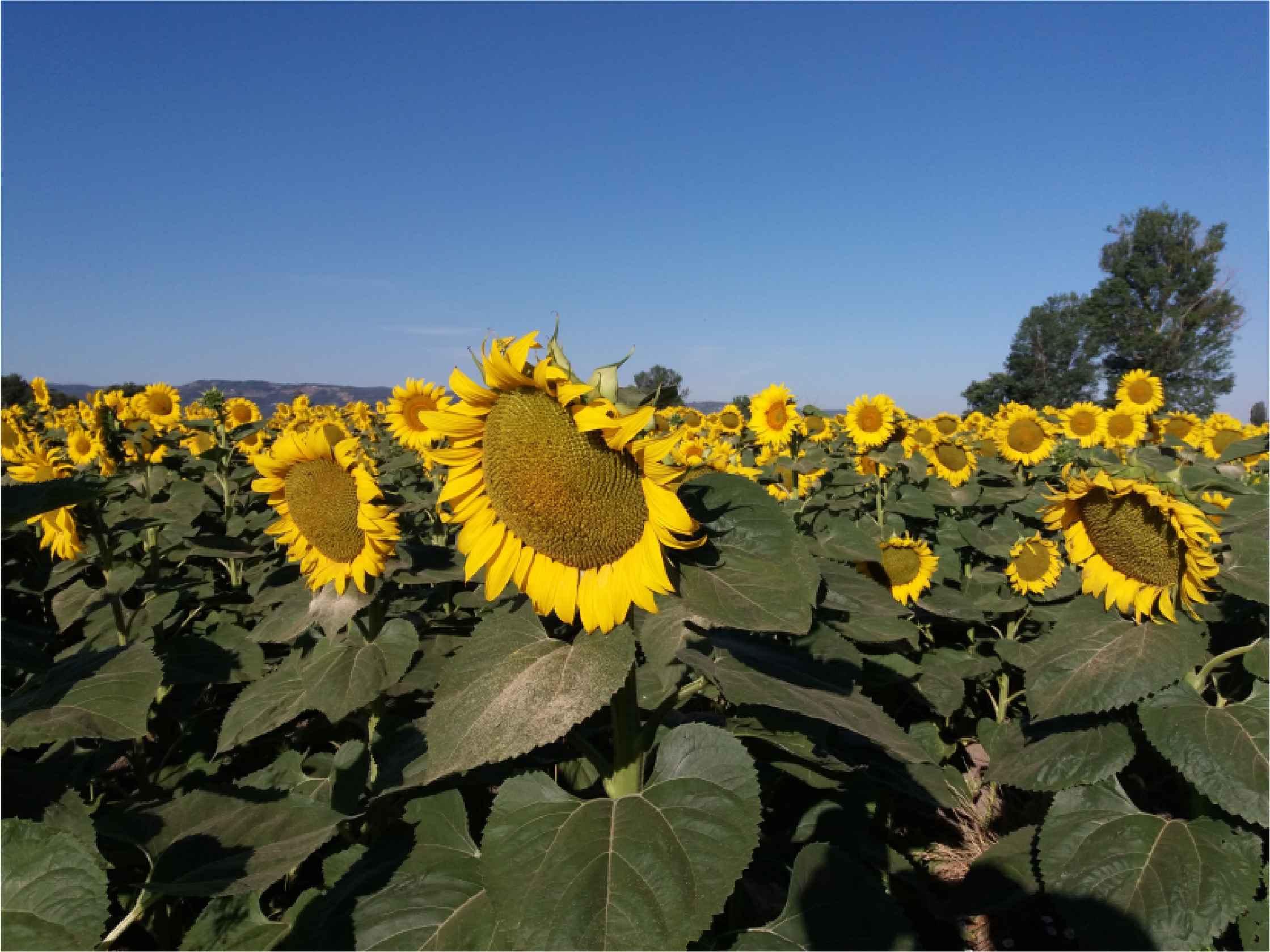
Sunflowers in Umbria.
Gabriel Lamé worked on the recurrent series un+2 = un+1 + un with initial conditions u0 = 0; u1 = 1, and for this reason it was known as the Lamé series. Notwithstanding the fact that various mathematicians had worked on this series, it was apparently only in 1876 that the name Fibonacci was linked to this recurrent series [69]. Lamé’s work with the series was purely mathematical, in contrast to superellipses, which he developed to deal with natural shapes, in particular crystals.
It is simply a method of recurrence and the starting pair of numbers determines the outcome. If this pair is (1, 1) or (1, 2) one obtains the Fibonacci series, the so-called main sequence of phyllotaxy. In the accessory series, the first side number is 1. Then the first pair of side and diagonal numbers (1, 3) will generate the numbers of the Lucas series (1, 3, 4, 7, …), also known as the first accessory series. The second and third accessory series start with (1, 4) and (1, 5) respectively. The so-called multijugate main sequence starts with (2, 4) leading to every term in the Fibonacci series doubled, namely 2 ⋅ (1, 1, 2, 3, 5, …). In the bijugate first accessory series the sequence is double of the Lucas series: 2 ⋅ (1, 3, 4, 7, …). And so on. Finally, the lateral sequences start with the side number 2 and for the first diagonal number odd numbers ≥ 5 are used (using 3 generates the Fibonacci series). This lateral sequence is also known as the anomalous phyllotaxis. Actually, the symmetry parameter in the Superformula can be a rational number, such as m = 5/2, generating a pentagram-like shape with five vertices closing in two rotations (Figure 57) giving the same as the Fibonacci 2/5 phyllotaxis.
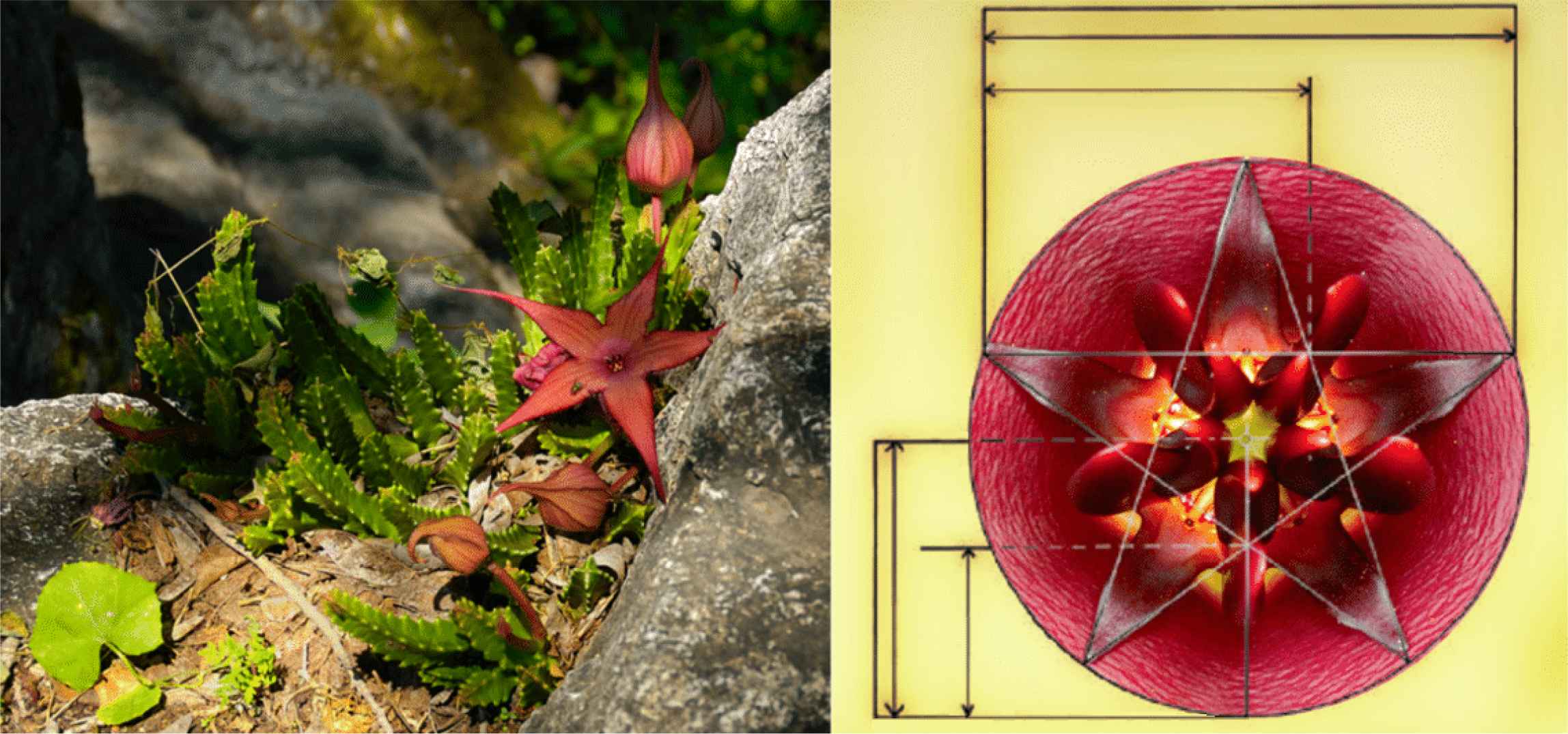
Pentagram symmetries in Huernia flowers.
Since leaves and scales on pinecones are discrete structures, one should look to difference equations, polynomials and logarithmic spirals to study phyllotaxy [41]. For example, Chebyshev polynomials, Lucas numbers Ln and Fibonacci numbers Fn can all be considered as special cases of the homogeneous linear second order difference equation with constant coefficients u0; u1; un+1 = aun + bun−1 for n ≥ 1. If a and b are polynomials in x, a sequence of polynomials is generated.
Particularly, if a = 2x and b = −1, we obtain Chebyshev polynomials. They are of the first kind Tn(x) for u0 = 1; u1 = x and of the second kind Un(x) for u0 = 1; u1 = 2x. Fibonacci numbers Fn arise for a = b = 1; u0 = 0; u1 = 1. For a = b = 1; u0 = 2; u1 = 1 we obtain Lucas numbers Ln. Therefore, if in Chebyshev polynomials
“Real analysts cannot do without Fourier, complex analysts cannot do without Laurent, and numerical analysts cannot do without Chebyshev. Moreover the mathematics of the connections between the three frameworks is beautiful.” [101]
For more information, please contact us at:
info@athena-publishing.com


