
From Pythagoras to Fourier and From Geometry to Nature
DOI: https://doi.org/10.55060/b.p2fg2n.ch012.220215.015
Chapter 12. Solution of Problems in Gielis Domains
Many applications of Mathematical Physics and Engineering are connected with the Laplacian:
The wave equation: utt = a2 Δ2u
Heat propagation: ut = κ Δ2u
The Laplace equation: Δ2u = 0
The Helmholtz equation: Δ2u + k2u = 0
The Poisson equation: Δ2u = f
The Schrödinger equation:
Boundary value problems relevant to the Laplacian are solved in explicit form only for domains with a very special shape, namely intervals, cylinders or domains with special (circular or spherical) symmetries [1]. In what follows, we limit ourselves to consider the extensions of classical problems to 2D normal polar domains of the Gielis type, that is domains
12.1 The Laplacian in Stretched Polar Coordinates
We introduce in the x, y plane the polar coordinates:
We introduce the stretched radius ρ* such that:
Therefore,
We show how to modify some classical formulas and we derive methods to compute the coefficients of Fourier-type expansions representing solutions of some classical problems. Of course, this theory can be easily generalized by considering weakened hypotheses on the boundary or initial data.
The case of the unit circle is recovered assuming ρ* = ρ and r(θ) ≡ 1. We consider a
We start representing this operator in the new stretched coordinate system ρ*, θ. Putting:
Using this polar equation, the corresponding stretched coordinates ρ*, θ in the plane x, y are given by:
For ρ* = ρ and R(θ) ≡ 1 we find the Laplacian in polar coordinates.
12.2 The Dirichlet Problem for the Laplace Equation in Gielis Domains
Consider the Dirichlet problem for the Laplace equation:
In [74] we have proven the result:
Theorem 12.1.
Putting:
the solution of the internal Dirichlet problem can be represented as:
Example
As an example, we start from the general Gielis equation [40]:
By assuming in Equation (12.12) that c = 22, α = 5, β = 8, m = 10, n1 = n3 = 6 and n2 = 4 we obtain the shape of the relevant domain
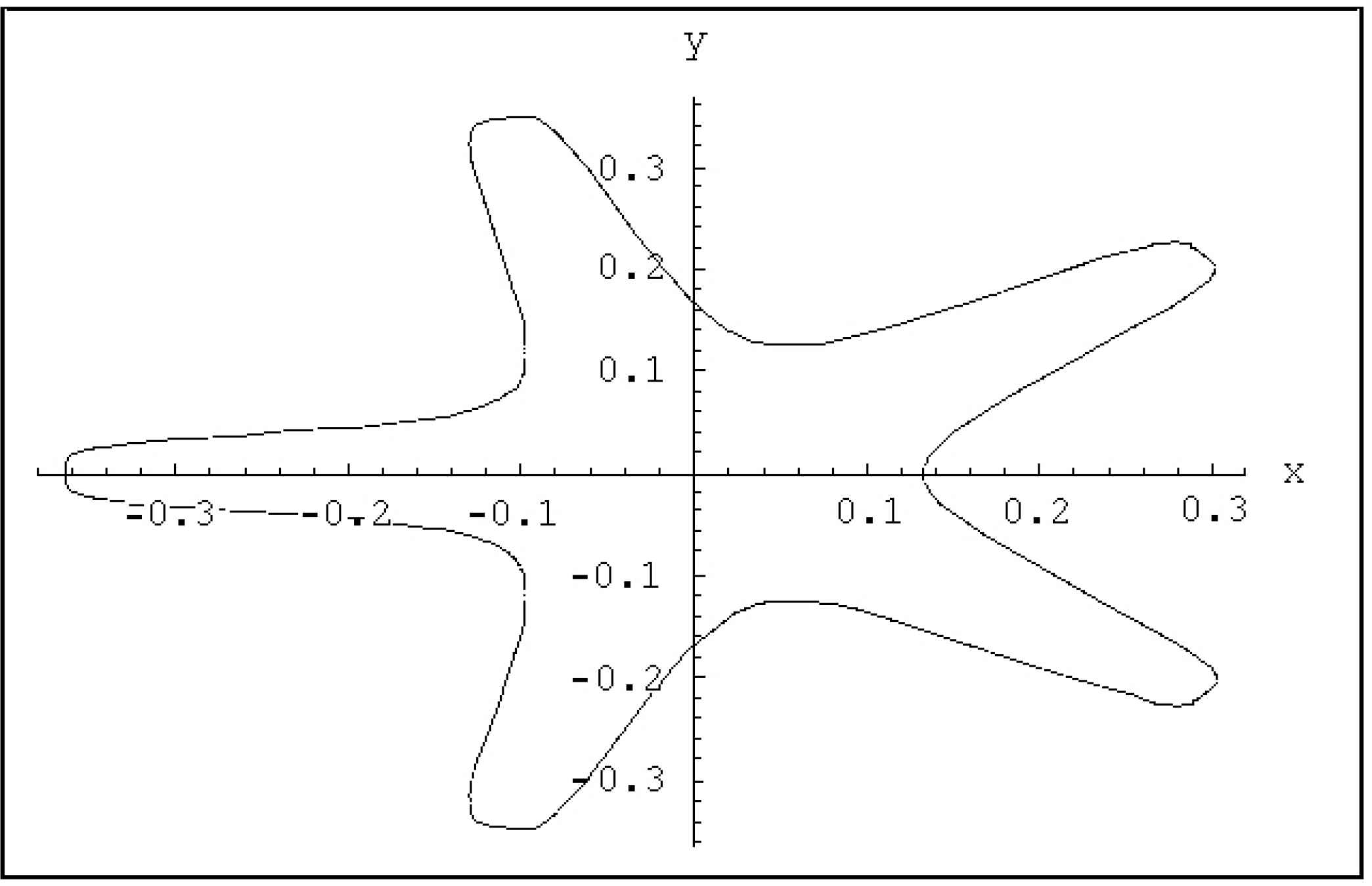
Starfish domain.
Let f(x, y) = cosh(x +y) + 5x2y be the function representing boundary values. Then we obtain the results reported in Table 3. In the first column we show the
| ∥f − u1∥L2 = 0.000335952 | ∥Δu1∥L2 = 0. × 10−17 |
| ∥f − u2∥L2 = 0.000133587 | ∥Δu2∥L2 = 0. × 10−17 |
| ∥f − u3∥L2 = 0.000101291 | |
| ∥f − u4∥L2 = 9.02500 × 10⁻⁵ | |
| ∥f − u5∥L2 = 5.42434 × 10⁻⁵ | |
| ∥f − u6∥L2 = 4.75581 × 10⁻⁵ | |
| ∥f − u7∥L2 = 4.75567 × 10⁻⁵ | |
| ∥f − u8∥L2 = 4.75565 × 10⁻⁵ |
L2 norms of boundary and inside approximation errors.
The obtained results, with P. Natalini as a coauthor (see [74]), show the convergence (in general a.e.) of the approximating sequence of functions to the function f, according to the general results on Fourier series proven by L. Carleson [22].
12.3 The Heat Problem in Gielis Domains
The heat problem for a plate with a general shape is often reduced to the circular case by using the conformal mappings technique (see e.g. [35, 65]), but only very special cases can be treated analytically by using this method since only few explicit equations for the relevant conformal mappings are known. However, it is possible to use the stretched coordinates system in order to obtain a quite general result for a Gielis domain.
Consider a plate with normal polar shape
In [73], with P. Natalini and R. Patrizi as coauthors, the following result was proven:
Theorem 12.2.
The above heat problem admits a classical solution:
Putting U (ρ, θ, 0) = F (ρ, θ) ≕ G(ρ*, θ) where:
Remark 3.
Note that the above formulas still hold if the function r(θ) is a piecewise continuous function and if the initial data are given by square integrable functions, not necessarily continuous, so that the relevant coefficients αh, βh in Equation (12.15) are finite.
Example
In the following example we consider, for the starlike plate, a Gielis equation of the type:
By assuming in (12.18) that c = 0.015, α = 12, β = 4, m1 = 12, m2 = 6, n1 = 8, n2 = 12 and n3 = 6, we obtain the shape of the relevant domain
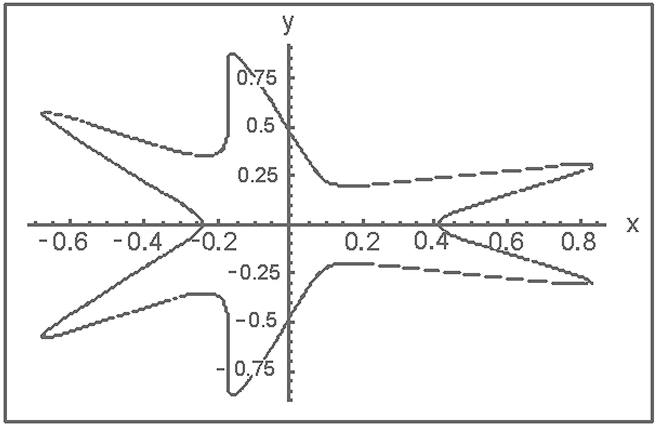
Shape of the domain
Let κ = 1.5 be the constant representing the diffusivity and f(x, y) = sinh(xy)+log(x2y2+1) the function representing the initial temperature. In Table 4, the
| t = 0 | 0.172694 | 5.87219 × 10−37 |
| t = 1 | 101.478 | 5.70500 × 10−48 |
| t = 2 | 1.48269 × 10⁻⁷ | 5.09531 × 10−58 |
| t = 3 | 5.87713 × 10⁻¹⁷ | 5.77811 × 10−68 |
L2 norms of boundary and inside approximation errors at different times.
In Figure 40 are shown, at time t = 0, the approximating solution u30 and the initial temperature f, both expressed in polar coordinates.
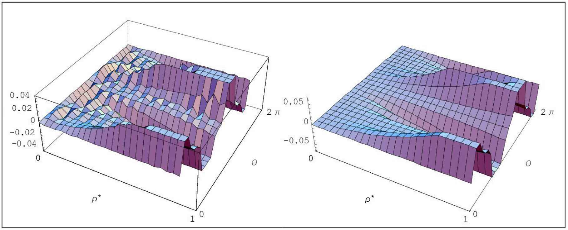
The approximating solution u30 and temperature f at time t = 0.
Remark 4.
We note that when the boundary values have wide oscillations, it is necessary to increase the number N of terms in the relevant Fourier expansion in order to obtain better results.
Remark 5.
The L2 norm of the difference between the exact solution and its approximate values is always vanishing in the interior of the considered domain and generally small on the boundary. Point-wise convergence seems to be true on the whole boundary, with the only exception a set of measure zero, corresponding to cusps or quasi-cusped points (i.e. regular points of the curve such that in a very small neighborhood the tangent makes a rotation of almost 180°). In these points, oscillations of the approximate solution (recalling the classical Gibbs phenomenon) usually appear. Therefore, the theoretical results of L. Carleson [22] are confirmed, even in the considered case.
12.4 The Wave Equation in Gielis Domains
Let us consider a membrane with normal polar shape
In [16], with D. Caratelli and P. Natalini as coauthors, the following result was proven:
Theorem 12.3.
Let:
Example
In the following example we assume for the boundary
By assuming in (12.28) that γ1 = γ2 = 3/4, p = q = 7, ν0 = 10, ν1 = ν2 = 6 and ϑ ∈ [0, 2π], the domain
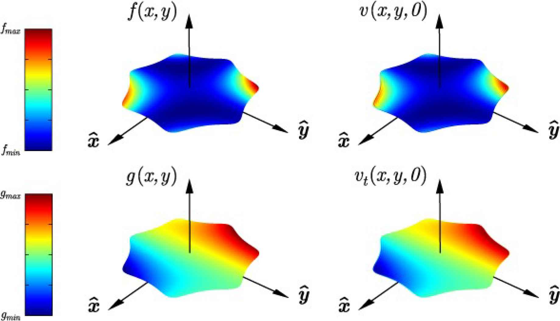
Initial distributions of displacement (top) and velocity (bottom) within the equisetum-shaped domain
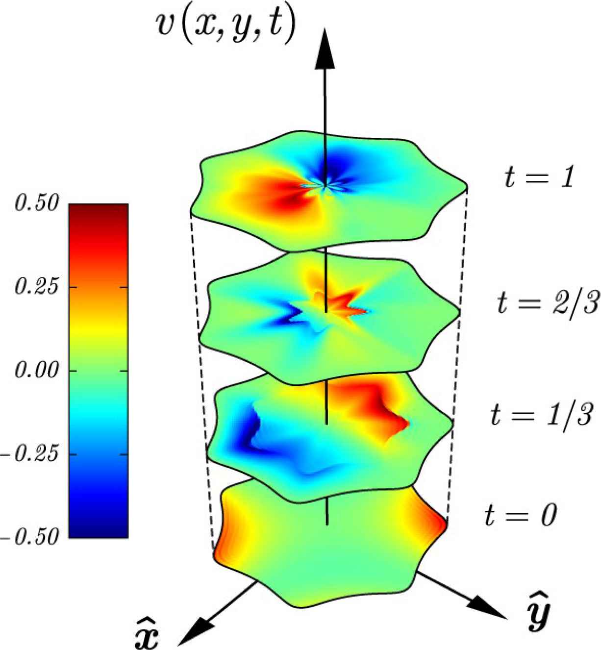
Spatial distribution of the displacement v (x, y, t) within an equisetum-shaped domain
Let
| eM,K | M = 0 | M = 30 | M = 60 |
|---|---|---|---|
| K = 1 | 99.325% | 74.383% | 74.382% |
| K = 30 | 91.050% | 15.745% | 15.744% |
| K = 60 | 90.612% | 4.291% | 4.239% |
For more information, please contact us at:
info@athena-publishing.com


