
From Pythagoras to Fourier and From Geometry to Nature
DOI: https://doi.org/10.55060/b.p2fg2n.ch001.220215.004
Chapter 1. The Pythagorean Theorem and Its Extensions
The Pythagorean theorem has its roots in the remote past. Early traces can be found in ancient Indian, Egyptian and Mesopotamian cultures, as the basis for the construction of the right angle necessary for the construction of buildings. In reality, the Pythagorean triples of integers (3,4,5), (6,8,10), (12,16,20), etc. first appeared and only later with the introduction of irrational numbers, attributed to the Pythagoreans themselves, its extension was considered, for example, through Theodore’s spiral.
The historical figure of Pythagoras himself is shrouded in mystery, as his birth on the Greek island of Samos has sometimes been questioned. It seems that he came to Magna Graecia and lived in Crotone, where he allegedly assumed political office and was subsequently killed in Metaponto during a revolt. None of this is certain. It is the figure of a philosopher who seems to have had strange metaphysical beliefs, such as that of metempsychosis, and was sometimes mocked for this reason (Horace, Satires, II, 6).
In any case, the importance of the theorem is fundamental in mathematics because it is linked to the concept of orthogonality which has so much relevance in modern mathematics. The extensions of the theorem to Euclidean spaces first, and more generally to those of Hilbert spaces, are recalled in the following as a basis for arriving at the series expansions of orthogonal functions introduced by Fourier series theory.
There exist many proofs of the Pythagorean theorem, starting with the one by Euclid. Here we use probably the most simple one, which makes use of the binomium square and the comparison of the areas of two figures, both shown in a geometrical way. No further comments are necessary.
In Figure 1 binomial square (a + b)2 = a2 + 2ab + b2 is proven.
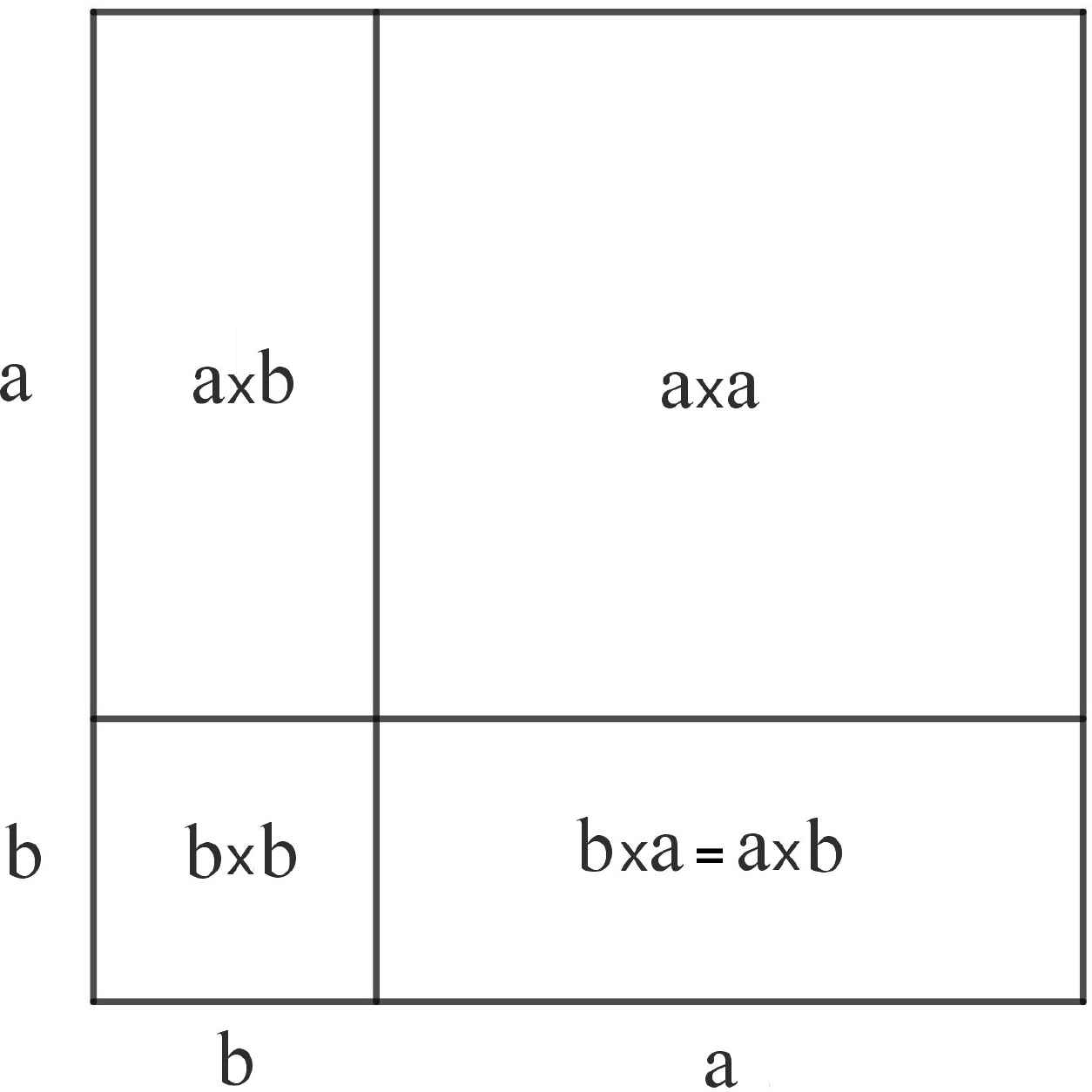
The square of a sum.
In Figure 2 a geometrical proof of the Pythagorean theorem is shown. The area of the square of side (a + b) is calculated in two ways: in the left figure as c2 + 2ab and in the right figure as a2 + b2 + 2ab. Since the areas are equal it must be a2 + b2 = c2.
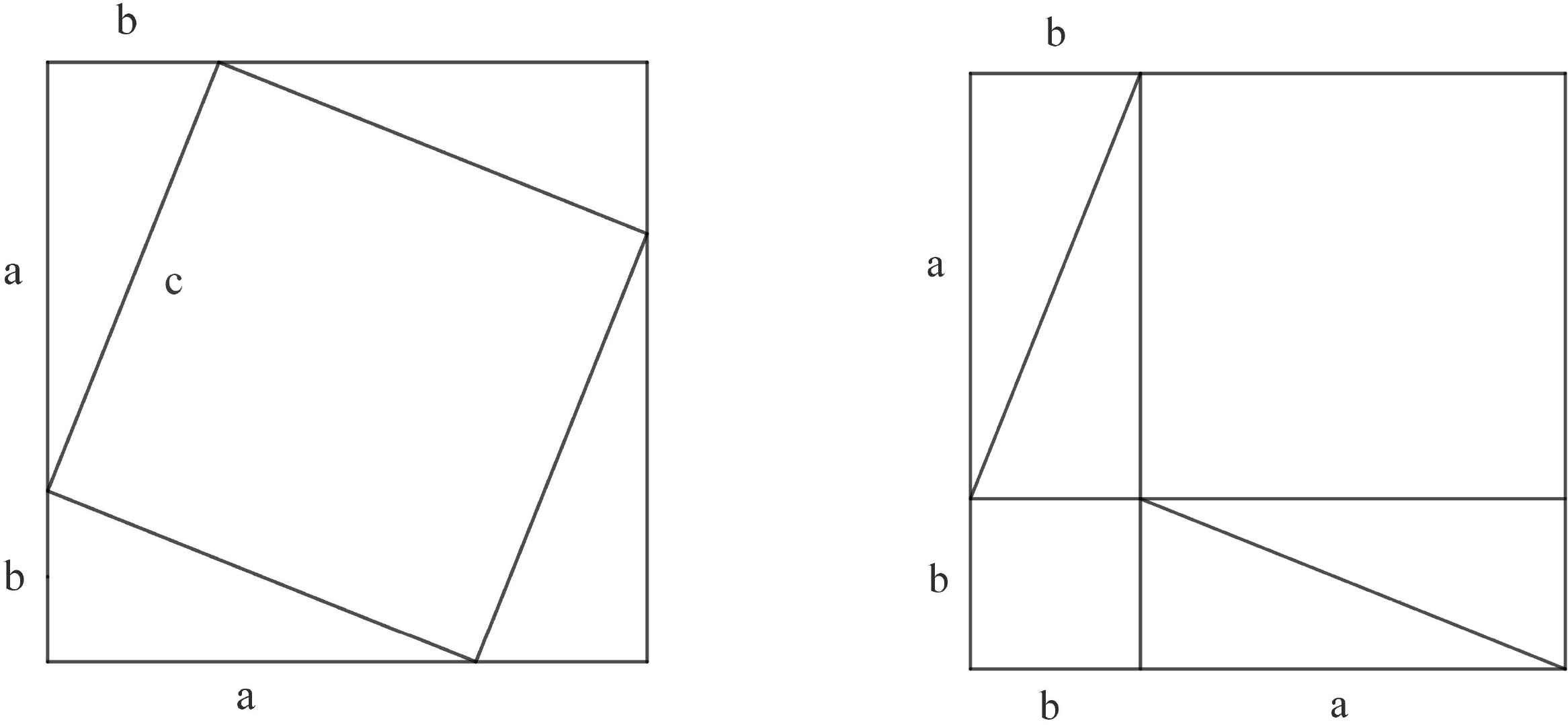
A geometrical proof.
1.1 Al-Kashi (Carnot) Theorem
An extension of the Pythagorean theorem known as the Carnot theorem was actually known by the Persian mathematician al-Kashi (1380-1429) [8]. It is also called the law of cosines. It results from applying the Pythagorean theorem, but it is necessary to distinguish two cases depending on whether the angle α = Â is acute or obtuse.
We refer to the case in which α is acute, so that | cos α| = cos α. In the other case, cos α < 0 but the minus sign in the following equation must be replaced by a plus sign so that both cases follow using the absolute value of cos α. Considering Figure 3, we have AD = b | cos α|, CD = b sin α, DB = c − b | cos α|, and by applying the Pythagorean theorem to the triangle DBC it follows that:
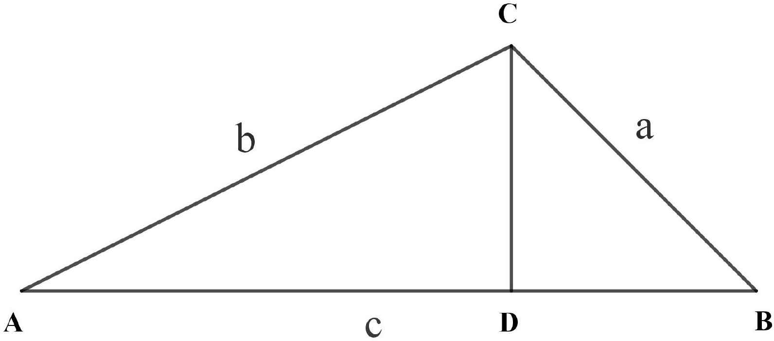
The case when α ≔ Â is acute.
1.2 Vector Space on R; Scalar Product in R2
A vector space V on R is an abelian group, with respect to the sum, of v elements called vectors [57]. This means that there is an associative and commutative sum operation. There is a null vector 0 such that ∀v ∈ V, v + 0 = v and for each v there is an opposite −v such that v + (−v) = v − v = 0. Moreover, it is possible to multiply the vectors by the numbers (called scalars) of R so that ∀u, v ∈ V, ∀α, β ∈ R, the following properties are satisfied:
The scalar product in R2 associates with each pair of elements of V an element (scalar) of R2 so that ∀u, v ∈ V, ∀α, β ∈ R, the following properties hold:
For calculation there are two definitions:
Putting:
In Figure 4 the geometrical meaning of the scalar product is shown.
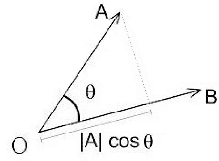
Meaning of the scalar product when
Equivalence of the two definitions
Given the vectors u = (u1, u2), v = (v1, v2), and denoting by |u| the length of the vector u, using the Carnot theorem it follows that:
1.3 Extension to Rn; Weighted Scalar Product
The definition of scalar product extends to the case of Rn by setting:
The following properties hold:
Bessel inequality in Rn:
Pythagorean theorem in Rn:
A further extension of the scalar product is obtained by introducing a weight vector w = (w1, w2, … , wn). Therefore, we define the scalar product with weight w by setting:
The notion of linear dependence and independence is of fundamental importance.
Definition. The vectors v1, v2, … , vm are linearly independent if and only if the following implication holds:
Otherwise, they are said to be linearly dependent. The linear combinations of the linearly independent vectors v1, v2, … , vm generate a linear manifold of dimension m:
Definition. The vector space V has dimension n if n is the maximum number of linearly independent vectors in it.
Introducing in the vector space V, of dimension n, the orthonormal base:
Then the vector u writes as:
In fact, we have:
For more information, please contact us at:
info@athena-publishing.com


