
Accepted 7 December 2020
Available Online 18 December 2020
- DOI
- https://doi.org/10.2991/gaf.k.201210.002
- Keywords
- Generalized trigonometry
generalized Fourier analysis
approximation of piece-wise linear functions - Abstract
Considering the diamond, i.e. the square inclined at an angle of 45°, it is possible to define the analogues of circular functions and to construct formulas that translate the trigonometric ones. The relative D-trigonometric functions have geometric shapes closely related to the corresponding classical ones, so that the orthogonality property can also be proven and D-Fourier expansions follow easily. Possible applications can be found in the representation piece-wise linear functions in a simpler way form compared to ordinary Fourier analysis.
- Copyright
- © 2020 The Author. Published by Atlantis Press B.V.
- Open Access
- This is an open access article distributed under the CC BY-NC 4.0 license (http://creativecommons.org/licenses/by-nc/4.0/).
1. INTRODUCTION
According to the work of Johan Gielis book [1], Mladinić [2] shows the possibility to introduce a trigonometry based on different geometrical shapes, generalizing the circle. Actually it should be possible, starting, for example, from a regular polygon centred at the origin, to introduce functions similar to the trigonometric sine and cosine and to find the equations that generalize the circular formulas. However, in order to recover the analogues of the simplest classical equations, it is necessary to choose the exact position of the polygon adjusted appropriately. This is not done in the above mentioned article [2], and this is probably why no equation is found in that article.
Among the considered figures, it seems that the most simple one is the diamond, defined by the parametric equations
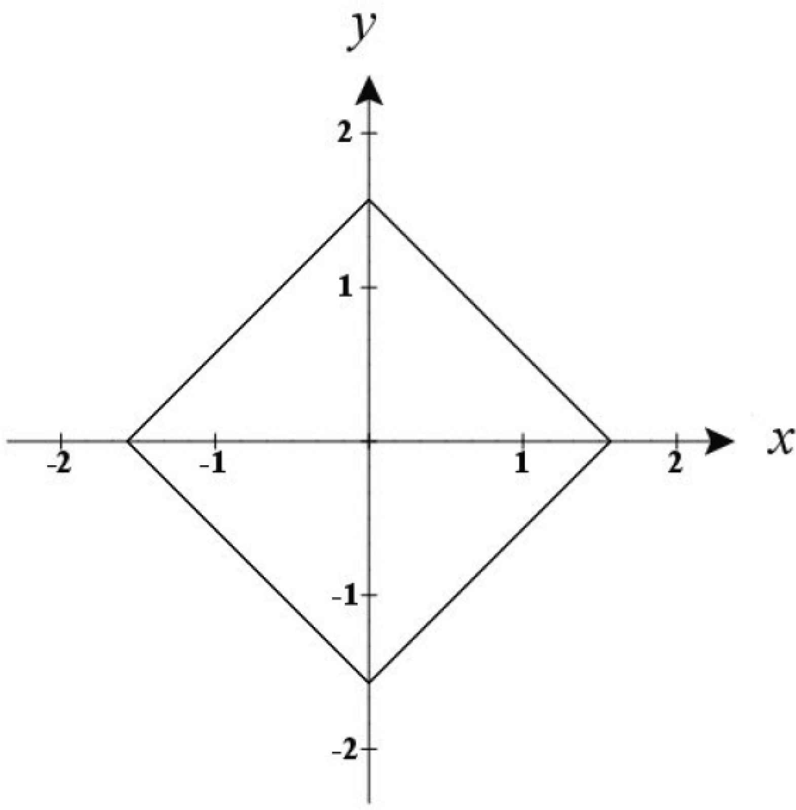
The diamond.
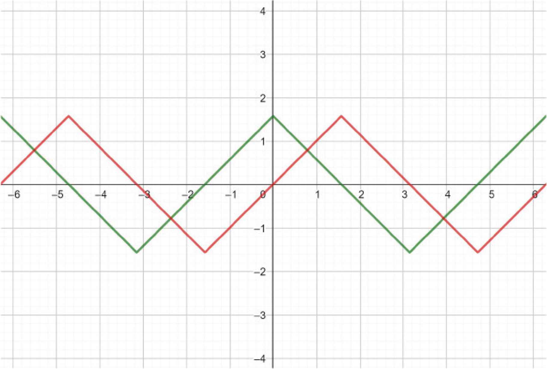
Green: x(t), red: y(t).
Actually the diamond is a very particular case (for n = 1) of the Lamé curves, as considered in Gielis [1].
Note that the basic equation sin(π /2 − t) = cost turns into
This is a fundamental property that is not valid for the graphs introduced in Mladinić [2], and which allows to build most of the results proved in the following.
2. BASIC GRAPHS
In this section we show the basic shapes of the D-trigonometric functions, noting the strict analogy with that related to the circle. A number of figures are reported in what follows, in order to justify this statement.
For example, we find the same periodicity for the functions in which the angle is a multiple or a submultiple.
- •
The periodicity of the functions arcsin(sin mt) and arcsin(cos mt) is 2π /m.
- •
The periodicity of the functions arcsin(sin(t/m)) and arcsin (cos(t/m)) is 2mπ.
Furthermore, the areas delimited by the graphs behave in a very similar way. This fact has an immediate effect on the calculation of the corresponding integrals and allows to determine the relevant orthogonality properties.
All these facts are shown in what follows, mainly by the graphical point of view, also noting that the considered functions are related with the possible motion of a bycicle with square wheels on a suitable ground, as it is recalled in [3].
Changing the angle into a its multiple, the graphs of functions exhibit the same character of the circular functions.
In what follows some examples are shown.
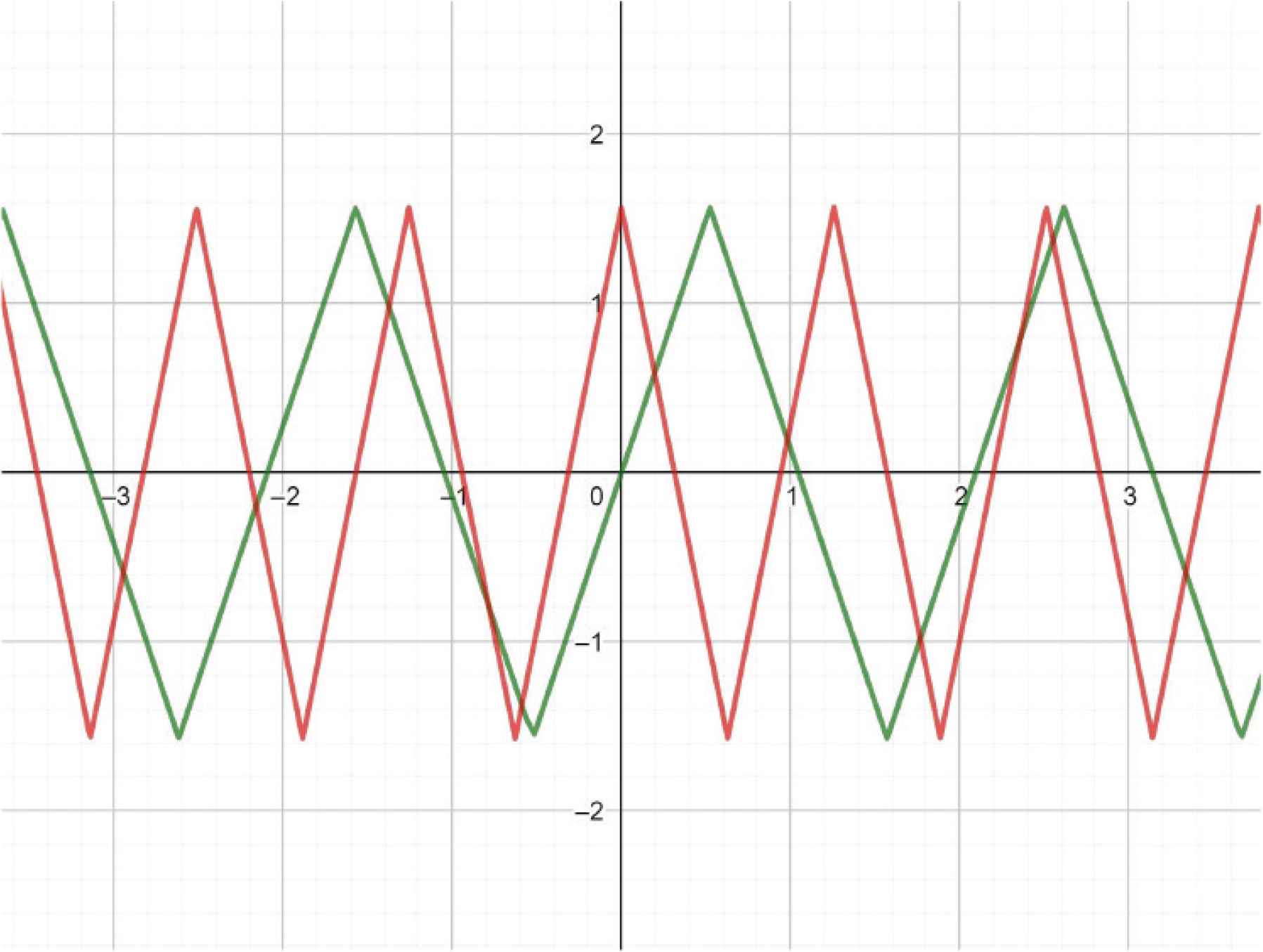
In Figure 3 the graph of arcsin(sin (3t)) is represented in green, and that of arcsin(sin (5t)) is represented in red.
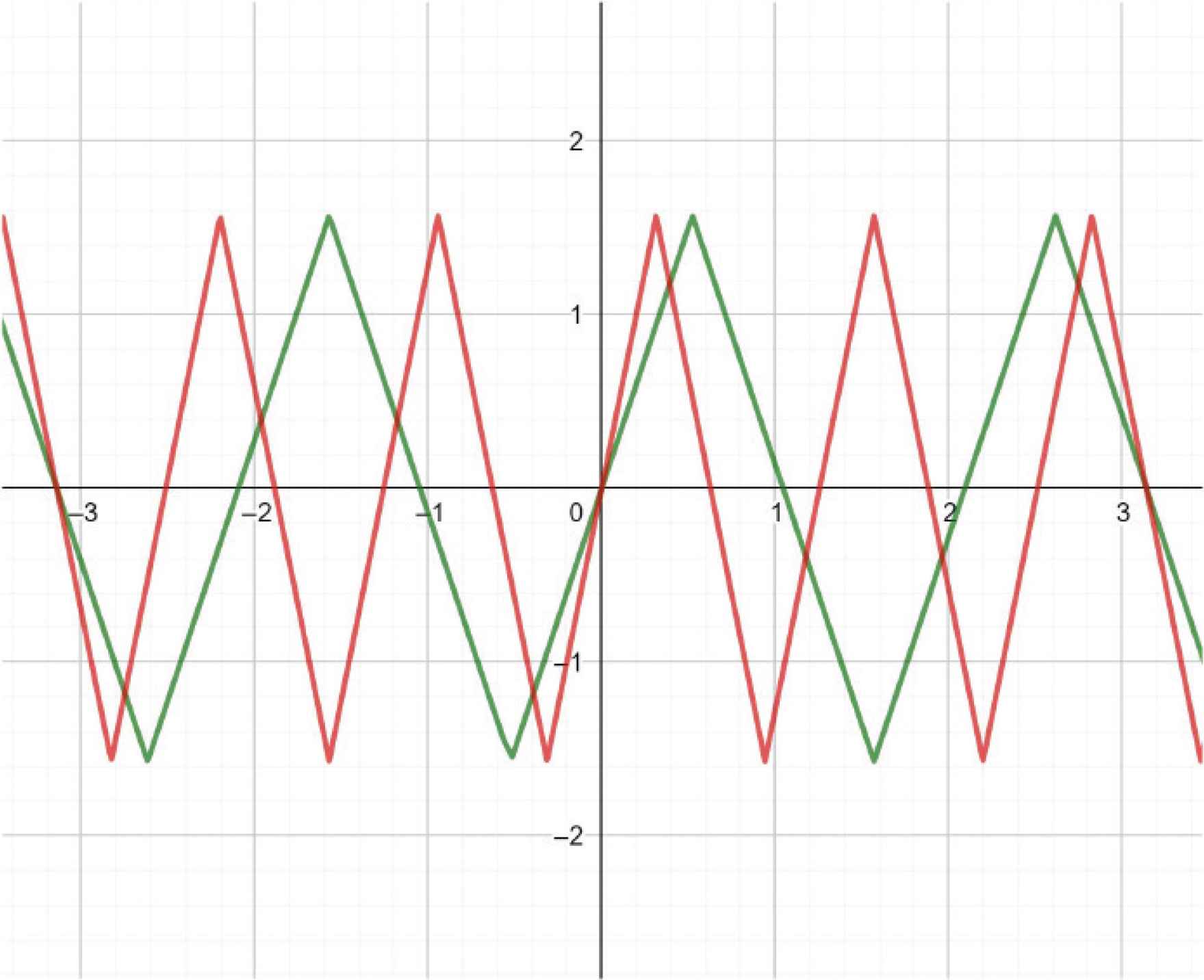
Green: arcsin(sin(3t)), red: arcsin(sin(5t)).
In Figure 4 the graph of arcsin(cos (3t)) is represented in green, and that of arcsin(cos (5t)) is represented in red.
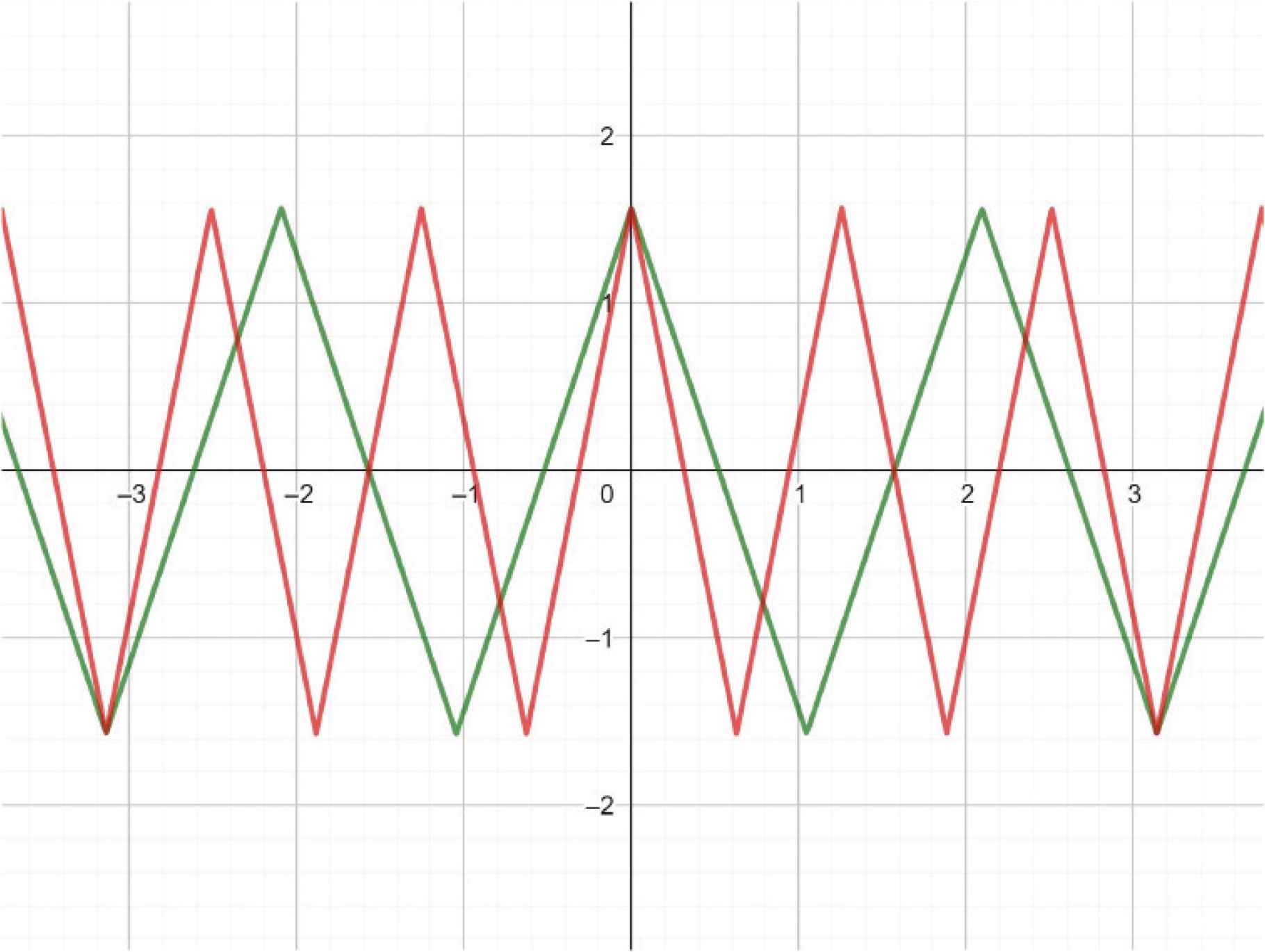
Green: arcsin(cos(3t)), red: arcsin(cos(5t)).
In Figure 5 the graph of arcsin(sin(3t)) is represented in green, and that of arcsin(cos(5t)) is represented in red.
Green: arcsin(sin(3t)), red: arcsin(cos(5t)).
In Figure 6 the graph of arcsin(sin(t)) is represented in green, that of arcsin(sin(2t)) in red and that of arcsin(sin(t/2)) in light blue.
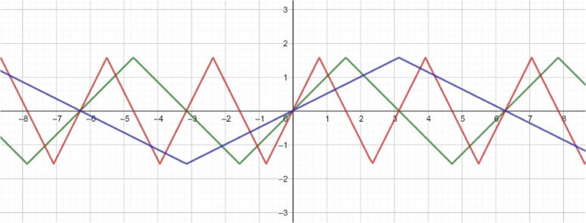
Green: arcsin(sin t)), red: arcsin(sin(2t)), blue: arcsin(sin(t/2)).
In Figure 7 the graph of arcsin(cos(t)) is represented in green, that of arcsin(cos (2t)) in red and that of arcsin(cos(t/2)) in light blue.
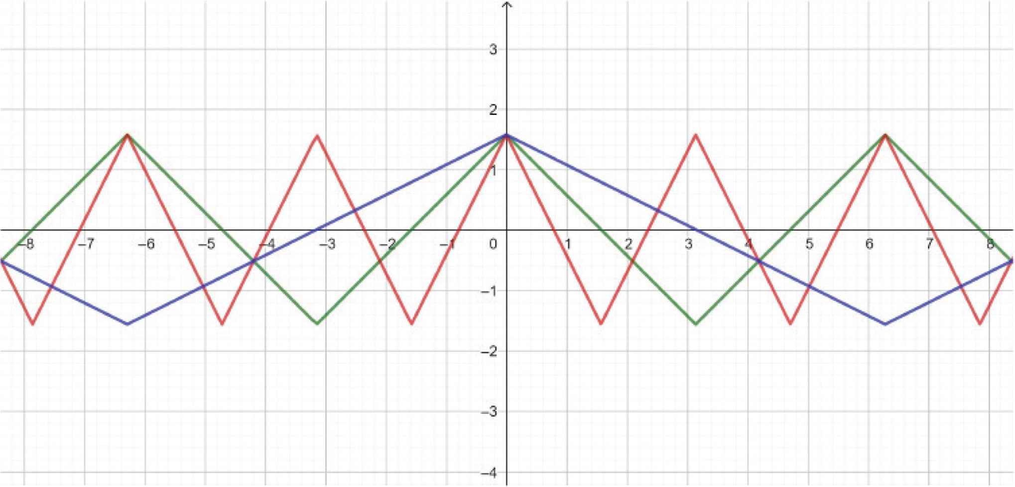
Green: arcsin(cos t)), red: arcsin(cos(2t)), blue: arcsin(cos(t/2)).
In Figure 8 it is shown the analogy with the circular tan and cotan functions.
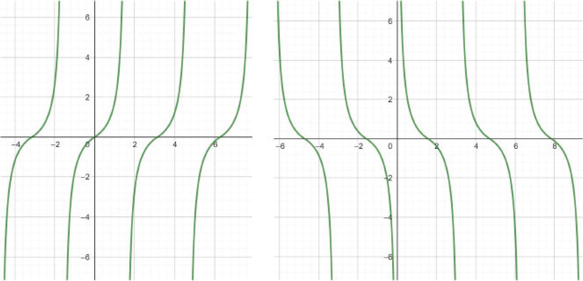
arcsin(sin t)/arcsin(cos t).
In Figure 9 it is shown the fundamental identity arcsin(sin2(t)) + arcsin(cos2(t)) = D(t), where D(t) is a periodic function similar to the type of profile under which the diamond can roll without crawling Derby SJ, et al. [3]. For the circle this profile is obviously a straight line (in the graph y(t) ≡ 1).
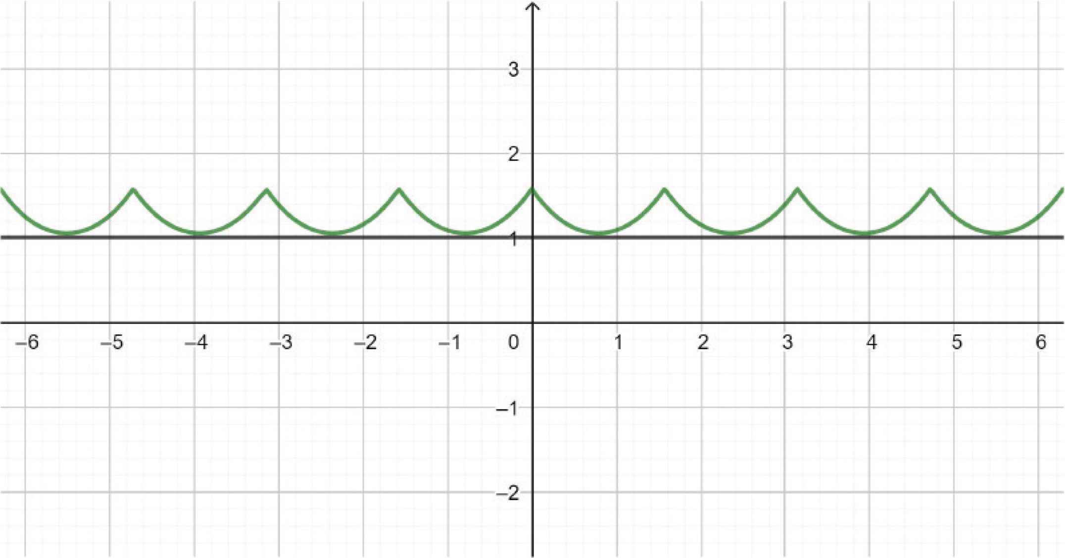
Green: arcsin(sin2t)+ arcsin(cos2t).
3. ANALOGY WITH THE CIRCULAR MULTIPLICATION FORMULAS
In Figure 10 we compare the two functions:
- •
arcsin(sin(2t)), in green,
- •
2arcsin(sin(t))arcsin(cos(t)), in red.
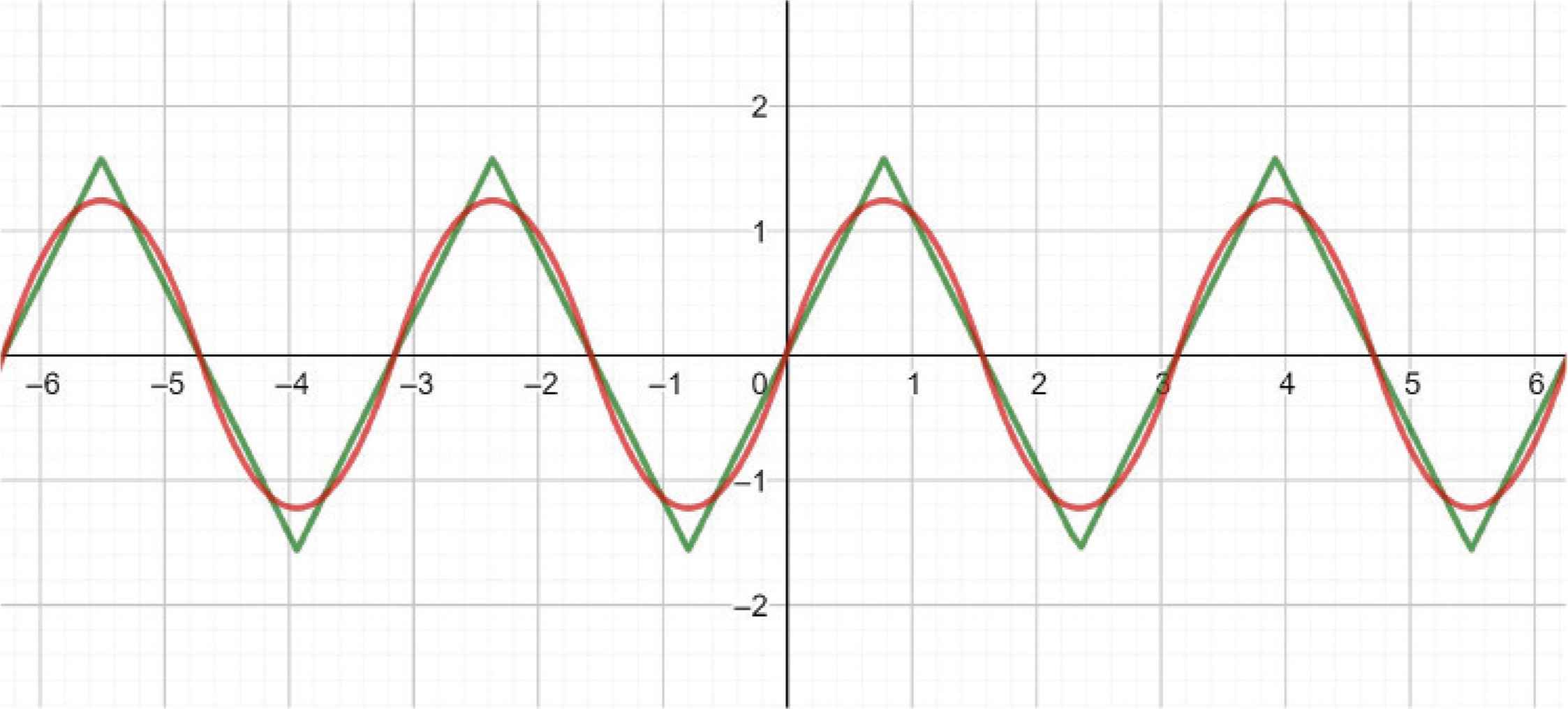
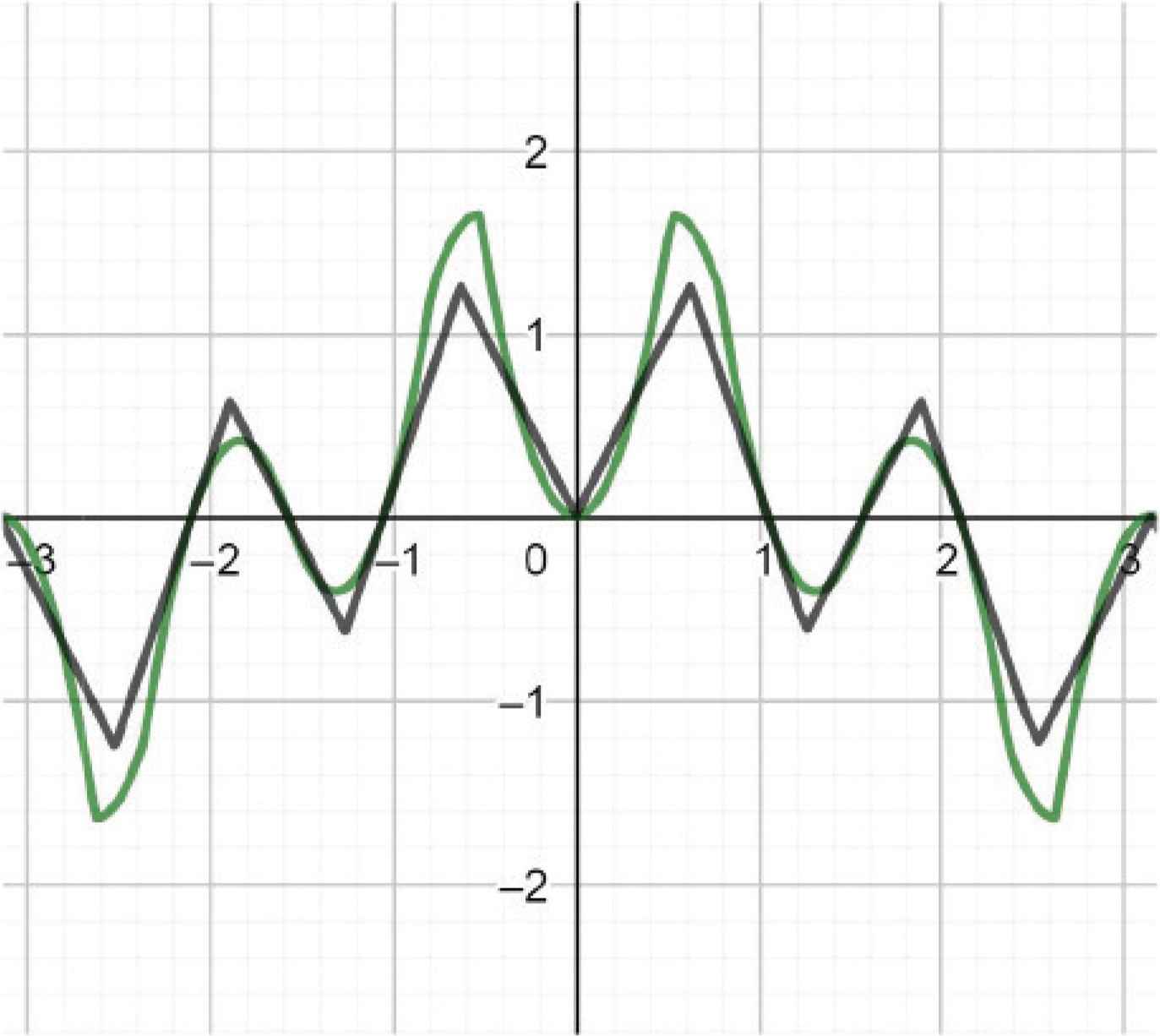
Green: arcsin(sin(2t)), red: 2 arcsin(sin(t)) arcsin(cos(t)).
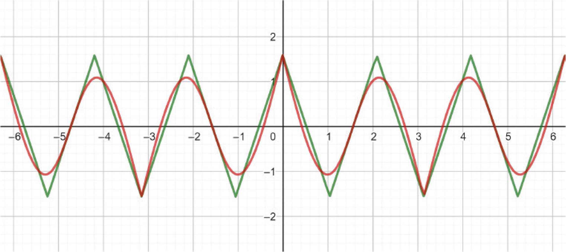
In Figure 11 we compare the two functions:
- •
arcsin(cos(2t)), in green,
- •
2arcsin(cos2(t)) − arcsin(sin2(t)), in red.
Green: arcsin(cos(2t)), red: 2arcsin(cos2(t)) – arcsin(sin2(t)).
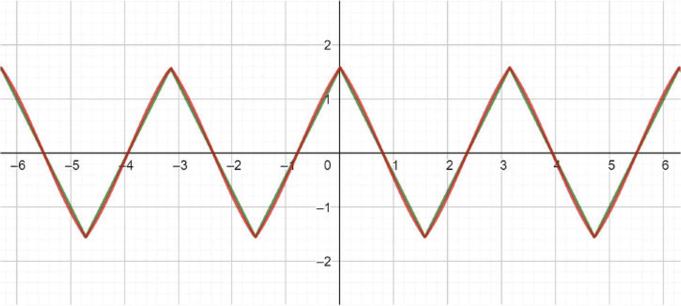
In Figure 12 we compare the two functions:
- •
arcsin(cos(3t)), in green,
- •
4arcsin(cos3(t)) − 3arcsin(cos(t)), in red.
Green: arcsin(cos(3t)), red: 4arcsin(cos3(t)) – 3 arcsin(cos(t)).
4. ANALOGY WITH THE CIRCULAR FORMULAS OF PROSTAFERESIS
In particular cases it is possible to show the analogy of the circular prostaferesis formulas [4] with those of the diamond case.
In Figure 13 the graphs of the functions
- •
arcsin(sin 3t) arcsin(sin 2t), in green
and
- •
are compared, showing the analogy with the circular equation
Green: arcsin(sin 3t) arcsin(sin 2t), black: 1/2 [arcsin(cos t) − arcsin(cos 5t)].
In Figure 14 it is shown the even function, representing the difference
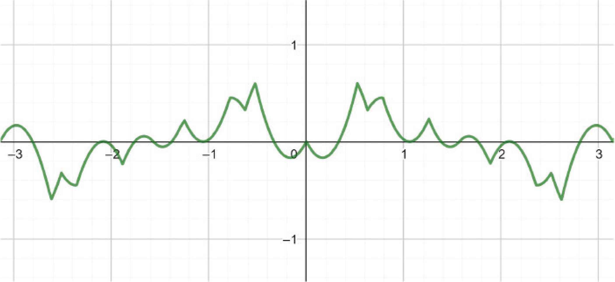
arcsin(sin 3t) arcsin(sin 2t) − 1/2 [arcsin(cos t) − arcsin(cos 5t)].
In Figure 15 the graphs of the functions
- •
arcsin(cos 5t) arcsin(cos 2t), in green
and
- •
are compared, showing the analogy with the circular equation:
Green: arcsin(cos 5t) arcsin(cos 2t), red: 1/2[arcsin(cos 7t) + arcsin(cos 3t)].
In Figure 16 it is shown the even function, representing the difference

arcsin(cos 5t) arcsin(cos 2t) − 1/2[arcsin(cos 7t) + arcsin(cos 3t)].
In Figure 17 the graphs of the functions
- •
arcsin(sin 4t)arcsin(cos 3t), in green
and
- •
are compared, showing the analogy with the circular equation
Green: arcsin(sin 4t) arcsin(cos 3t), red: 1/2 [arcsin(sin 7t) + arcsin(sin t)].
In Figure 18 it is shown the odd function, representing the difference
arcsin(sin(4t)) arcsin(cos(3t)) − 1/2[arcsin(sin 7t) + arcsin(sin t)].
5. ORTHOGONALITY PROPERTIES
The orthogonality of the functions arcsin(sin nt) and arcsin(cos mt), ∀ m, n is a trivial consequence of the symmetry of the interval and the odd symmetry of the product, so that:
It is also possible to prove the orthogonality properties, ∀ n ≠ m:
To this aim, it is sufficient to observe that the orthogonality property of the circular functions, that is ∀ m ≠ n, the definite integral in (−π, π) of the products cosmt cosnt or sinmt sinnt follows from the graph of these functions, for which the positive values of the areas above the t axis are compensated, by symmetry, by the negative values below.
Since the products arcsin(cos mt)arcsin(cos nt) and arcsin(sin mt)arcsin(sin nt) are piece-wise linear functions which exhibit a high variation in the considered interval, the numerical computation, by considering all sub-intervals in which the function is linear, is not possible in general. However, it is possible to compare the product arcsin(cos mt)arcsin(cos nt) with cos mt cos nt and the product arcsin(sin mt)arcsin(sin nt) with sin mt sin nt. A graphical comparison, for every fixed m and n, will prove the same behaviour of the two functions.
A few particular examples are shown below, but the same result can be checked for every different values of m and n, in order to prove the orthogonality of functions for these values.
Let us consider here some special cases.
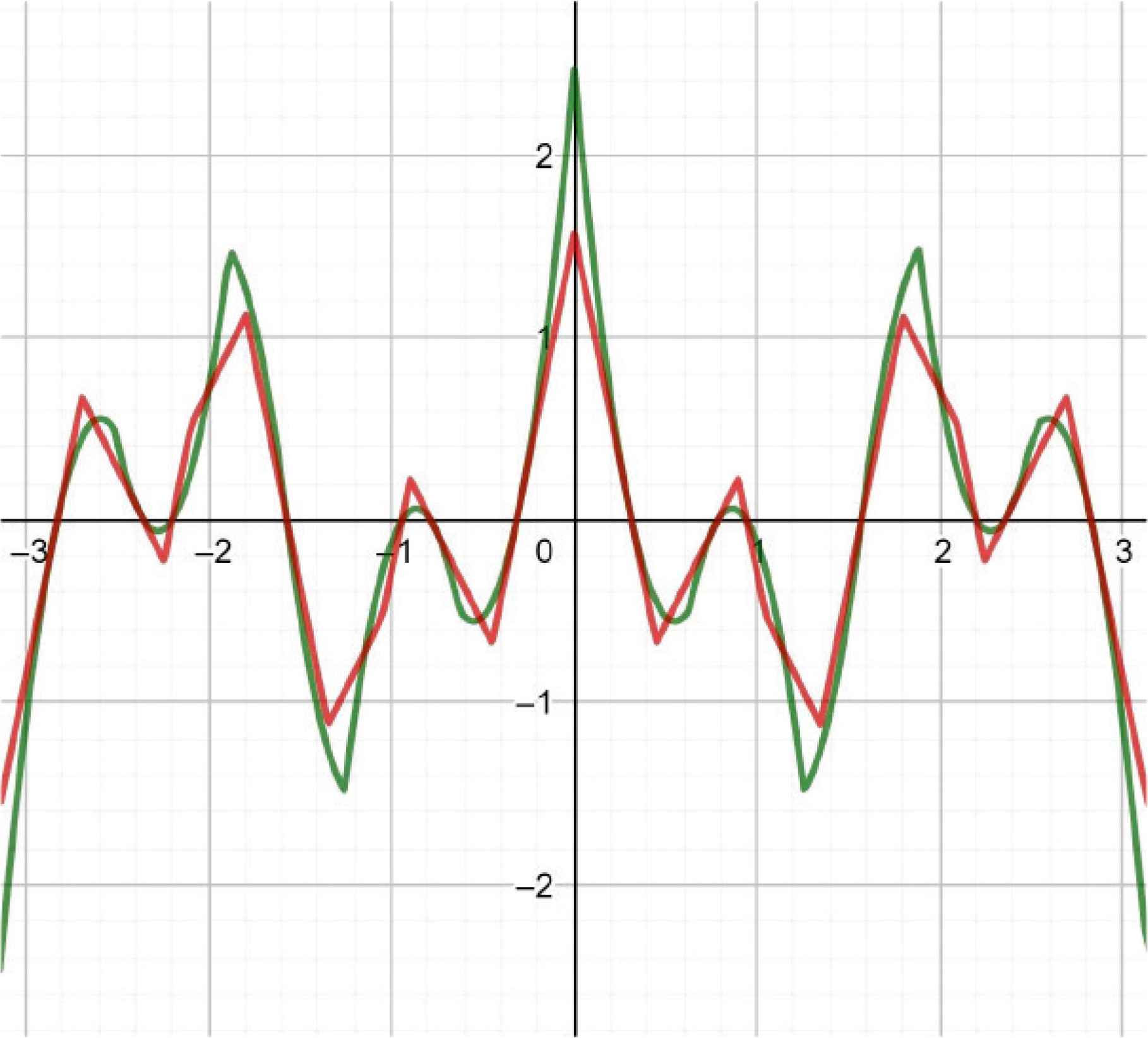
In Figure 19 (left) the graph of the function cos(2t)cos(7t), in green, is compared to that of arcsin(cos(2t))arcsin(cos(7t)), in red.
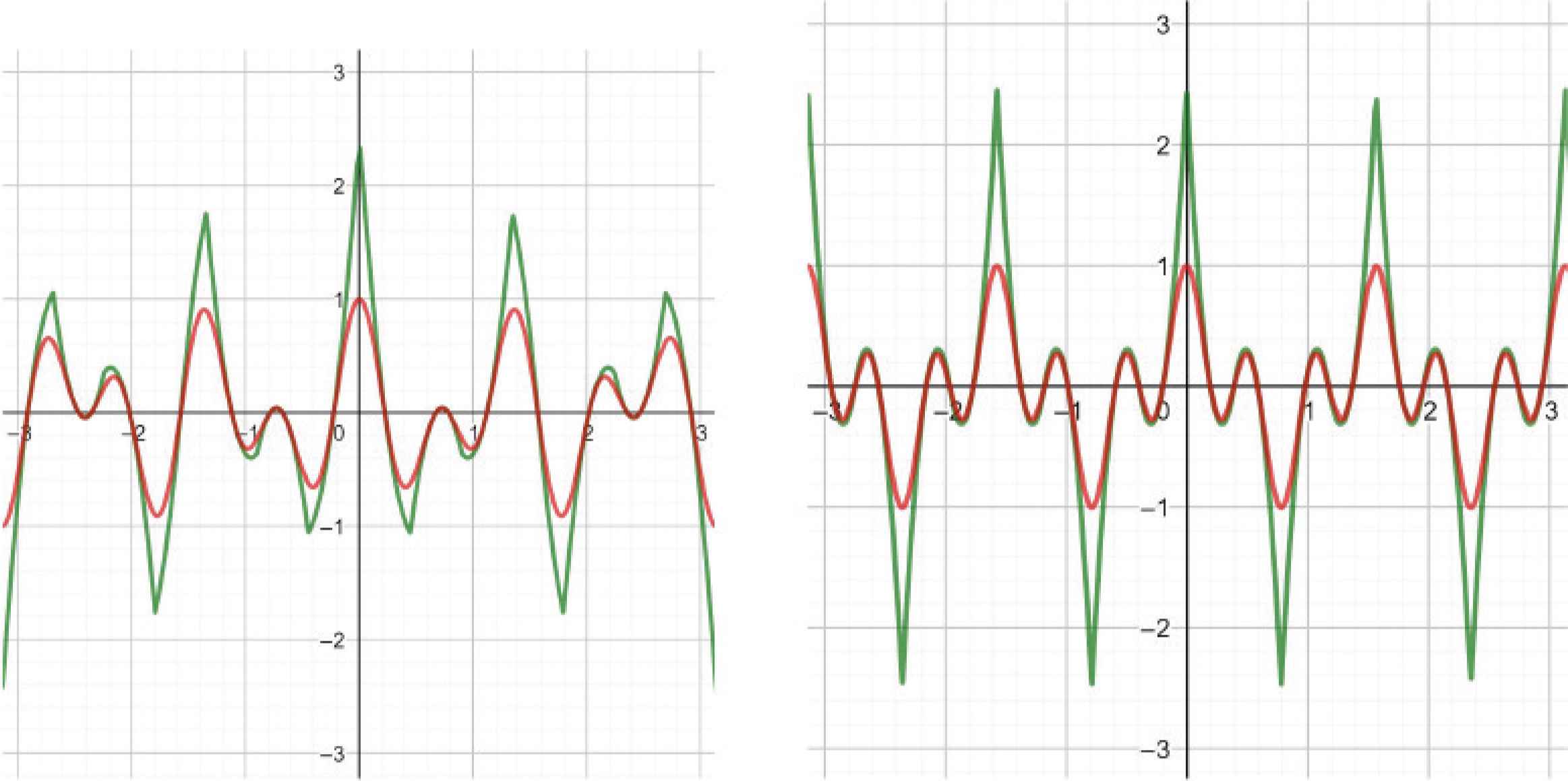
Left: cos(2t) cos(7t), in green VS arcsin(cos(2t)) arcsin(cos(7t)), in red; right: cos(4t) cos(8t), in green VS arcsin(cos(4t)) arcsin(cos(8t)), in red.
In Figure 19 (right) the graph of the function cos(4t)cos(8t), in green, is compared to that of arcsin(cos(4t))arcsin(cos(8t)), in red.
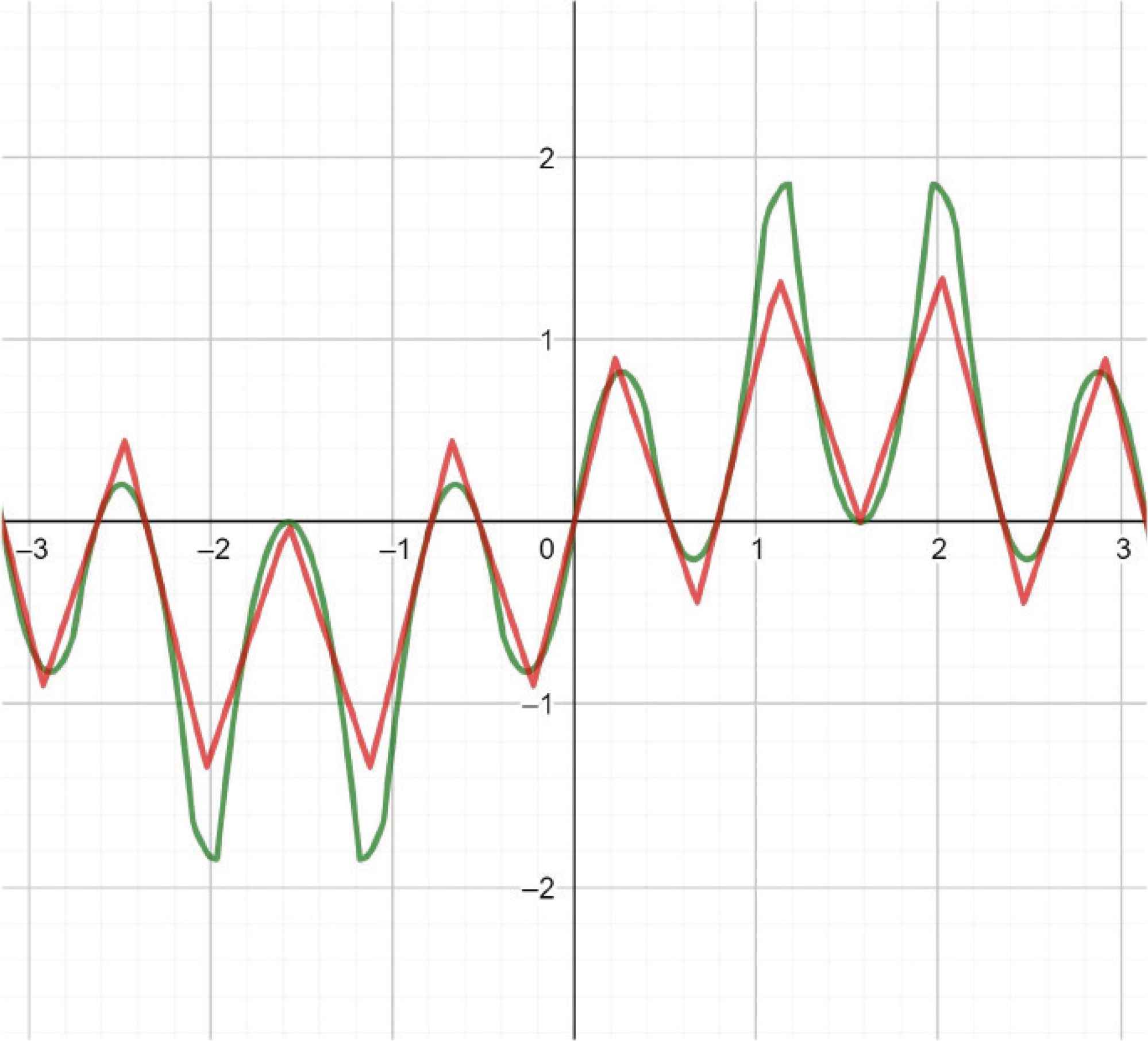
In Figure 20 (left) the graph of the function sin(2t)sin(4t), in green, is compared to that of arcsin(sin(2t))arcsin(sin(4t)), in red.
Left: sin(2t) sin(4t), in green VS arcsin(sin(2t)) arcsin(sin(4t)), in red; right: sin(4t) sin(5t), in green VS arcsin(sin(4t)) arcsin(sin(5t)), in red.
In Figure 20 (right) the graph of the function sin(4t)sin(5t), in green, is compared to that of arcsin(sin(4t))arcsin(sin(5t)), in red.
6. EXAMPLES OF D-TRIGONOMETRIC POLYNOMIALS
Noting that by using combinations of the above considered functions, i.e. considering D-trigonometric polynomials, it is possible to represent with a closed form many piece-linear functions that are usually expressed by trigonometric series. A few examples are shown in the figures below.
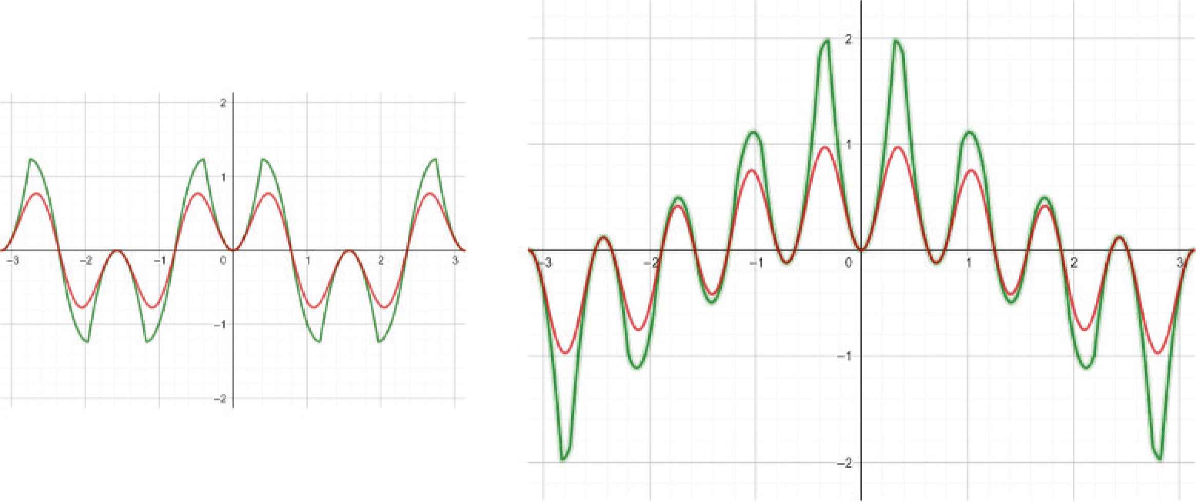
In Figure 21 (left) it is shown the graph of function
Left: arcsin(sin(2t)) + arcsin(cos(2t)), right: arcsin (sin(2t)) + arcsin(cos(3t)).
and in Figure 21 (right) the graph of the function
In Figure 22 (left) it is shown the graph of the function
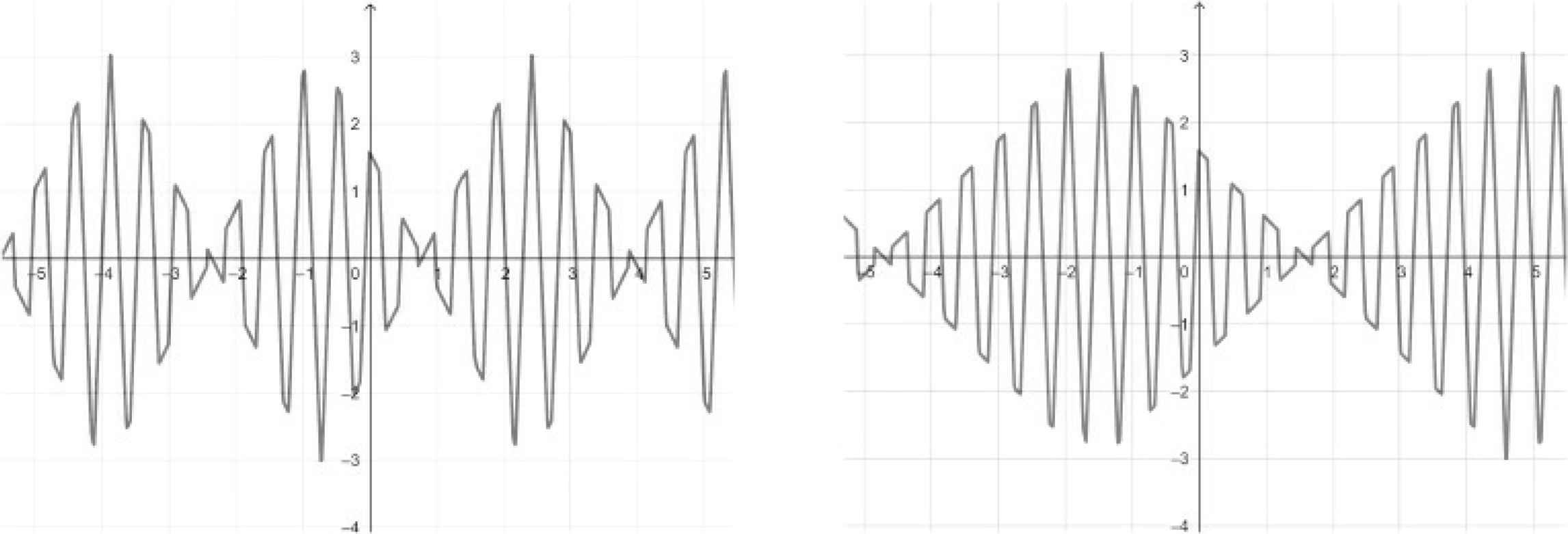
Left: arcsin(sin(11t)) + arcsin(cos(13t)), right: arcsin(sin(12t)) + arcsin(cos(13t)).
and in Figure 22 (right) the graph of the function
The shape of the combinations shown in the above figures suggests the possibility to represent graphs with high variation linear functions, typical of sounds or seismic phenomena, with D-Fourier series expansions, that is expansions in arcsin(cos t) and arcsin(sin t) functions.
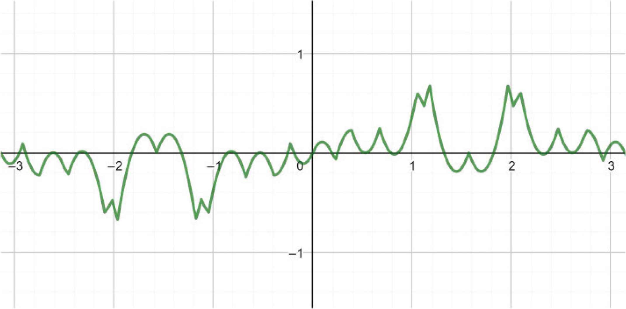
In Figure 23 (right) a sound wave, and in Figure 23 (left) the periodic function, combination of D-trigonometric functions:
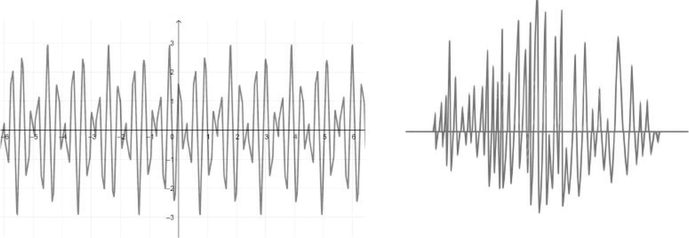
Left: arcsin(cos(21t))+ arcsin(sin(15t)), right: a sound wave.
7. D-FOURIER POLYNOMIAL EXPANSIONS
As it seems that only a small number of D-trigonometric functions are sufficient to approximate graphs of complicate shapes, in what follows we consider only D-Fourier polynomial expansions, avoiding the complicate problems of series’ convergence.
Given a function f(t) ∈ L2(−π, π), put:
Then the coefficients are computed by the using Fourier’s method [5].
For k = 0, by Eqs. (3) and (4), it results:
The integrals in the denominators of Eqs. (9) and (10) are given by:
Remark 7.1.
Note that for computing the integral in Eq. (11) it is necessary to divide the interval into several parts and to use the additivity property of the integral with respect to the integration set.
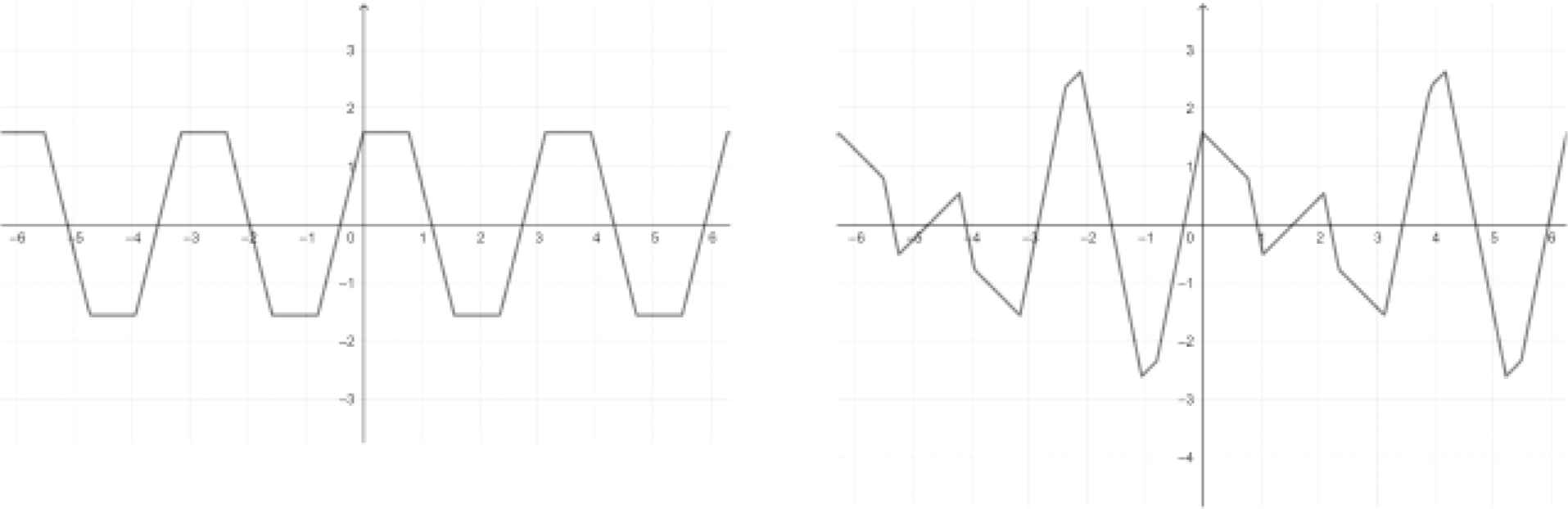
Two examples can be seen in the next figure, where the interval is divided into four and eight parts.
In Figure 24 the graphs of the functions arcsin(sin(2t))2, (on the left) and arcsin(sin(4t))2, (on the right), are shown.
Left: arcsin(sin(2t))2, right: arcsin(sin(4t))2.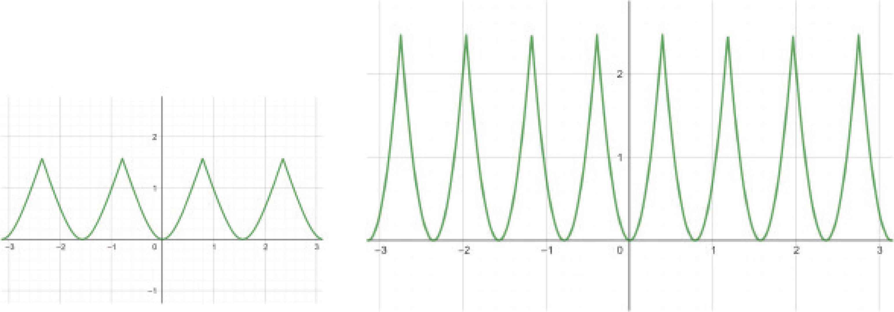
Then, introducing the constant D ≔ 5.16771…, we find:
Therefore, Eq. (5) writes:
8. CONCLUSION
The D-trigonometric functions, that is the analogues of the circular function, related to a diamond instead of a circle have been introduced. These functions exhibit a character strictly related to the classical trigonometric functions, and it is possible to write for them equations corresponding to the circular ones. Deriving the orthogonal properties, by exploiting the symmetry properties of the relevant graphs, the D-Fourier polynomial expansions can be easily proven. It is worth to note that finite combinations of D-trigonometric functions allow to write the piece-wise linear functions in a more simple way with respect to their Fourier expansions.
CONFLICTS OF INTEREST
The author declare that he has not received funds from any institution and that he has no conflicts of interest.
ACKNOWLEDGMENTS
I thank Dr. Johan Gielis for letting me know his book on the Circle and the article of Petar Mladinić that gave birth to this project.
REFERENCES
Cite This Article
TY  - JOUR
AU  - Paolo Emilio Ricci
PY  - 2020
DA  - 2020/12/18
TI  - A Note on the D-trigonometry and the Relevant D-Fourier Expansions
JO  - Growth and Form
SP  - 11
EP  - 16
VL  - 2
IS  - 1
SN  - 2589-8426
UR  - https://doi.org/10.2991/gaf.k.201210.002
DO  - https://doi.org/10.2991/gaf.k.201210.002
ID  - Ricci2020
ER  -


