
Revised 18 June 2021
Accepted 4 April 2022
Available Online 6 May 2022
- DOI
- https://doi.org/10.55060/j.gandf.220605.001
- Keywords
- Buckingham theorem
Dimensional analysis
Homogeneous functions
General relativity - Abstract
The theory of dimensions in physics is astonishingly rich. It can be viewed at different levels of abstraction and, at any of these levels, reveals deep suggestions. The relevant theory was initially developed to get a useful mean to reduce the number of variables in experiments. Within this context Rayleigh method and Buckingham Π theorem are highly conceptual working tools. Further elements of novelty have emerged during the last years and methods, directly or indirectly, linked to dimensional analysis, have become a central issue to treat families of differential equations, to enter deeply in the so-called scaling relations characterizing the phenomenology, not only in physics but in social science, economy, biology, and so on. This article is an effort aimed at providing a reasonably comprehensive account of the theory and the relevant practical outcomes, which spans over a large variety of topics including classical issues in hydrodynamics but also in general relativity and quantum mechanics as well.
- Copyright
- © 2022 The Authors. Published by Athena International Publishing B.V.
- Open Access
- This is an open access article distributed under the CC BY-NC 4.0 license (https://creativecommons.org/licenses/by-nc/4.0/).
1. INTRODUCTION
1.1. Dimensional Analysis and Reduction of Complexity
Any quantitative science relies on the necessity of introducing specific quantities to be defined through a measure, implying a protocol, tools and units. The geometry, if intended in its etymology γεωµητρια (measurement of land) is such an example. The measure itself may be intended through different procedures, the most natural of which is the comparison with a reference quantity. Regarding geometry, the length is what is intended to be specified in quantitative terms.
We define in abstract terms the geometrical dimension [L], which is a primitive concept, as stressed below. Such a concept is richer than it may appear and has evolved through the concept of dimension illustrated below.
The point has dimensions zero [L0], the line 1 [L1], the area 2 [L2] and the volume 3 [L3]. The reference quantity can be a unit sub-segment, a unit square a unit cube (see Fig. 1).
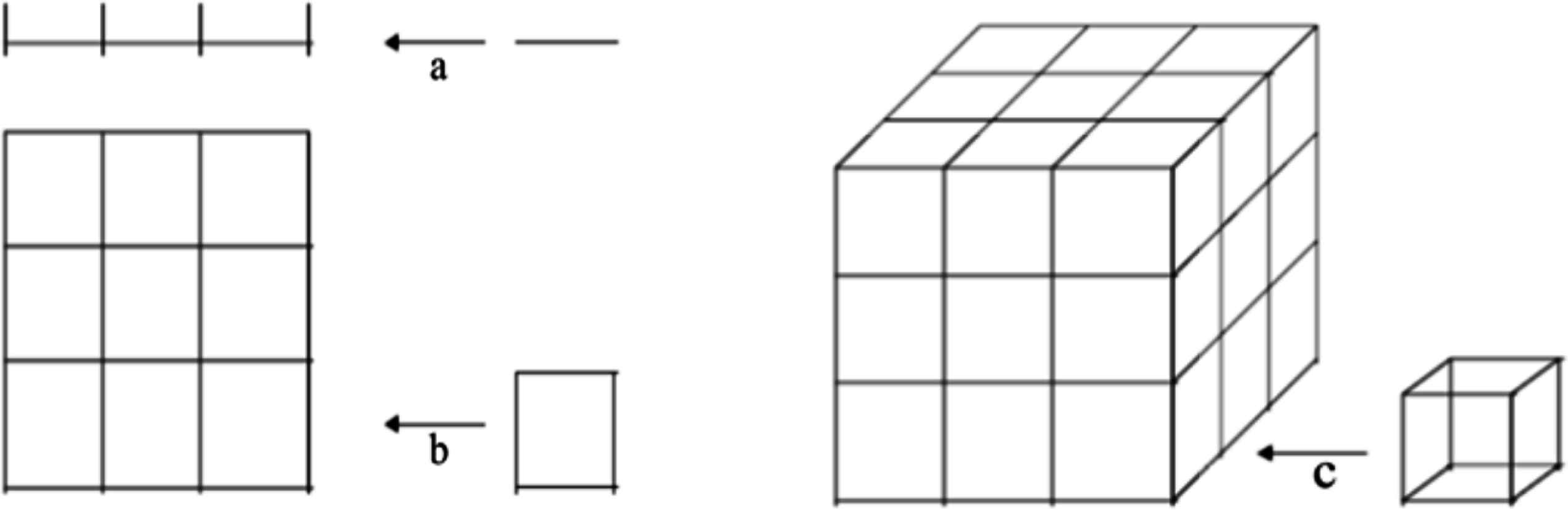
Elementary geometry dimensions: a) length, b) surface, c) volume.
What we have described so far is very elementary. According to this picture a length is just the sum of a certain number (3 in Fig. 1) of the chosen reference measure, say 3 s, if s is the reference measure. Accordingly surface and volume scale as 32, 33 respectively.
The essence of Physics is the experiment, which lies on the concept of measurement. A prerequisite for the process of measure is the development of a protocol, according to which one attributes a gauge to characteristic quantities, thus getting a numerical meaning for pure concepts, often referred as “fundamental” or “primary” dimensions (PD), like length [L], time [T] and mass [M], if we limit ourselves to mechanical problems.
Let us remain, for the moment, within the land of pure abstraction and think in terms of dimensions, without referring to any specific system of units. Any physical quantity like energy [E], velocity [U]1, force [F]. . . can be expressed as “dimensional products” of the aforementioned PD and for example, we find
The question arises on what fundamental does mean. In philosophical terms we may refer to length, time and matter as “pre-categories” through which “reality” can be organized within a deductive context.
We simply rephrase the point of view of the Kantian philosophy to state that L, T, M are the tools which are “triggered” by the experience to formulate “a priori analytical propositions” and transform perceptions into a “phenomenon”.
In principle perception in physics can be organized not only through what we have defined PD, but through other “means” as, for example, E, F, U. The idea we like to convey is that the meaning of “fundamental” is just a matter of convention, as shown below in an appropriate mathematical context.
In general, any mechanical quantity will be specified by the dimensional equation
Where α, β, γ are not necessarily positive and integers.
We provide an idea of how the process of assigning dimensions proceeds. An example is provided by the definition of the viscosity of a fluid, which can be viewed as its resistance to flow. The concept is illustrated in Fig. 2, where we have reported a liquid within two plates (with surfaces A), the upper of which moves and drags lamina of flow, whose velocity increases with the height (vertical direction in Fig. 2). We can accordingly state that the liquid resistive force is
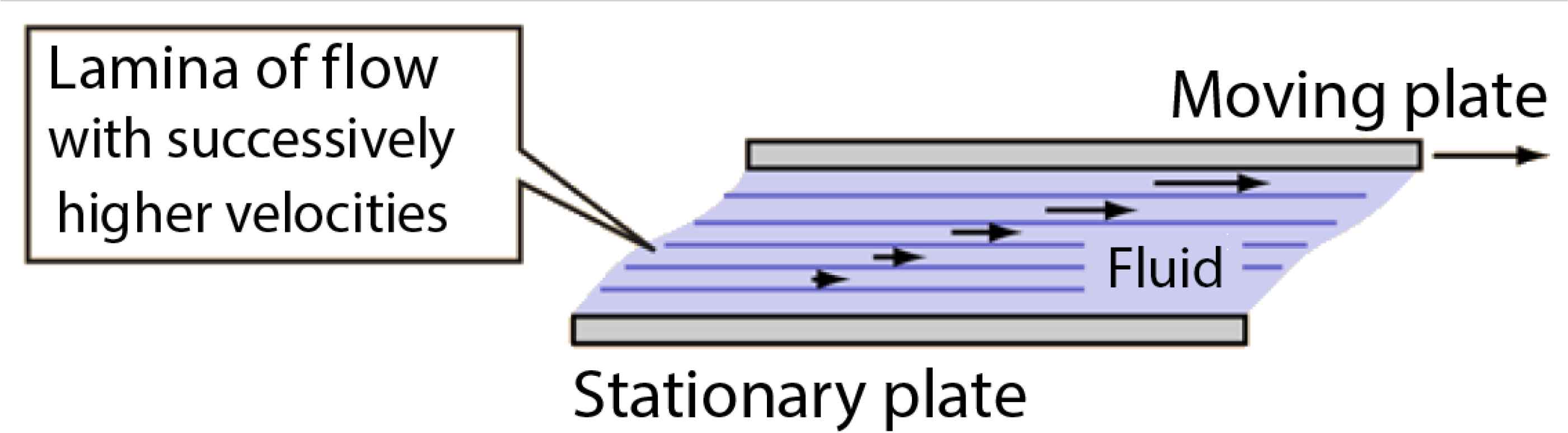
Schematic representation of fluid resistance.
The dimensional content of the coefficient μ is readily obtained
Before proceeding further, we make a step forward in the process of abstraction and define the “space of dimensions”, spanned by the unit vectors
In this space the quantity Q is written as
It is therefore worth noting that, keeping three linearly independent triples of primary units
They are invertible
Accordingly, the statement of fundamental and derived dimensions is, at least in mathematical terms, only matter of a choice, as discussed more accurately below and in the forthcoming sections.
For example, we find that by keeping energy, force and velocity as “fundamental”, the following dimensional correspondence with time, mass and length can be established
There is however nothing deep in what we have noted, which, said in these terms, is just a reshuffling of symbols, the forthcoming sub-section contains a more substantive step further.
1.2. Dimensional Analysis and the Principle of Homogeneous Dimensions
The topics and concepts, we have discussed so far, can be organized into what is recognized as dimensional analysis (DA), which provides a powerful mean to get a preliminary insight into the “scaling” of physical quantities, within a given phenomenological context.
It is worth to adding, as important premise, the Principle of Dimension Homogeneity, which, albeit tacitly assumed, is now explicitly worded as follows
All additive terms in a dimensional equation have the same dimensions
This statement clarifies the obscure wording (dimensional product), used before. We accordingly note that power is the ratio between work and time, work is the same as energy (at least in terms of dimensions), therefore we find
A paradigmatic example of application of DA is associated with the drag forces, emerging as consequence of the viscosity and we use dimensionality argument to guess an analytical form for the force itself. By analytical we mean how the various physical quantities defining the problem are embedded to get a force.
A preliminary analysis indicates that all the quantities of interest can be arranged as in the table shown below, where we have included velocity (U) Surface (S), density (ρ) and viscosity (μ) along with the relevant PD content.
On the right column we have added the force and the relevant dimensions to be matched.
We have four physical quantities and 3 primary dimensions. This gives us 4 choices to aggregate U, S, ρ, µ to end up with a force, one of which is shown below:
We can accordingly conclude that the force may be cast as
The factor
Eq. (11) is dimensionally correct, but we cannot exclude any proportionality coefficient, which can be expressed as function of a non-dimensional quantity emerging from the combination of the variables entering the definition of our problem.
To clarify this point and attempt a solution, we consider different arrangements of the reference quantities and assume that
Which leads to
Together with dimensional, non-dimensional quantities play a pivotal role in the analysis of physical phenomena. A non-dimensional quantity naturally emerges from Eq. (13) as the ratio between forces, i.e.
This is a non-trivial quantity and is recognized as the Reynolds number:
The other ratios yield
We have not developed any theory to specify how Re should be appended to the definition of force. We can however assume that Eq. (11) is true except that it should be multiplied by a not specified function of the Reynolds number, i.e.
The practical outcome of this discussion is that if we are interested to carry out an experiment to specify cd we are not obliged to perform four groups of different measures, but we can just study the behavior of 2F/(ρ v2 S) vs. Re.
From the discussion in this introductory section, Dimensional analysis emerges as a working tool useful to analyze a physical problem and getting scale relationships between wisely chosen groups of variables. A significant byproduct of the procedure is the identification of key quantities useful to reduce the complexity of the problem under study. This is certainly true, but we believe it is much more, as we will try to convey in the forthcoming sections.
2. THE BUCKINGHAM THEOREM AND ITS CONSEQUENCES
2.1. Ship Design and the Froude Number
In the previous section we have mixed up and anticipated different points, which we are going to develop in a more systematic way. We have mentioned the procedure of combining quantities like surfaces, density, viscosity and velocity to derive either the drag force and a non-dimensional number inferred as a byproduct of this melting criterion. The previous ideas trace back to the seminal works of Rayleigh [1,2] and Buckingham [3,4] which will be discussed below.
The Rayleigh method, even though brilliant, amounts to grouping a number of physical quantities, fix primer dimensions, combine the exponents and match them to another specific quantity. The procedure strongly relies on the principle of dimensional homogeneity, on experience and physical intuition as well.
To illustrate the method, an example is better than any comment. We ask therefore the following question: in a given physical phenomenon the velocity depends on the pressure [p] ≡ [ML−1T−2], and density [ρ] = [ML−3], can we use DA to guess the dependence of velocity on the previously quoted quantities?
To answer the question, we require that
Which, embedded into the dimensional vector space, yields the relation
The principle of identity between vectors (i.e. the dimension homogeneity condition), imposes that
We have “discovered” an obvious identity, which becomes only slightly less trivial, if we look at the problem from a different perspective, namely by asking whether DA can help us to infer the dependence of the velocity of propagation of a pressure wave through a liquid, in terms of its elasticity (K) and density. The use of the outlined procedure yields
The next example is the guessing of a dimensionless number (the Froude number) of central importance in the design of ships.
The analysis of the motion of ships during their traveling at sea, at lakes or at rivers is an extremely difficult problem. It should be therefore noted while traveling the boat-wave interaction usually determines the formation of steep diverging bow and stern waves, possibly breaking. Furthermore the ship geometry and the velocity are responsible for a complex phenomenology, as, for example, the generation of vorticity in the wave-breaking region, the appearance of free-surface scars, and the entrainment of air, to name a few [5].
To better appreciate the physical nature of the previously quoted phenomena and the relationship with the Reynolds number, we go back to fundamental principles.
A body in a fluid may be subject to different forces, including those of viscous
Accordingly we can write
Thus finding, from Eq. (11)
The discussion we have developed so far may appear simplistic, we will see at the end of the paper how the nondimensionalization of the Navier-Stokes equation leads to analogous conclusions.
2.2. The Buckingham Π Theorem
According to the previous discussion it has emerged that, in correspondence of a certain number of dimensional variables, there exist a number of non-dimensional quantities. It is therefore quite natural to specify how many of these numbers can be found in correspondence of the list of dimensional terms.
The answer is contained in an important theorem of dimensional analysis, proposed by Buckingham [3,4] and asserting that
“Given a list of n dimensional quantities with k primary units, the number of corresponding non dimensional products is n – k”
Or, in alternative form:
“A dimensionally homogeneous equation, involving n physical variables, all expressible in terms of k independent fundamental physical quantities, can be expressed in terms of p = n – k dimensionless parameters”
A preliminary example is certainly useful to clarify what the previous statements mean. We consider therefore the following problem, given an equation
Accounting for the dependence of F with the dimension of a force on
Namely a total of 6 variables. Because we have chosen M, L, T as primary dimensions (see below), we should be able of working out 3 non-dimensional parameters, characterizing the same equation. The above general formulation is sufficient to work out a solution, in any case if like a less abstract formulation, we can reformulate it in the following way [7]:
a thin rectangular plate having a width w and a height h is located so that it is normal to a moving stream of fluid. We can guess that the drag force, exerted by the fluid on the plate, depends on the plate dimensions (w, h), on the fluid viscosity and density (µ, ρ respectively) and on the velocity of the fluid approaching the plate. We can determine a suitable set of non-dimensional quantities (Π′s, see below) to study this problem experimentally.
The dimensional matrix, characterizing the problem is drawn below
Since we are looking for non-dimensional quantities, we proceed as follows.
The first step is the definition of a number of “repeating variables”3 to be embedded with the others to get the desired non-dimensional terms. The number of repeated variables are (usually) the same as the primary dimensions, we choose (w, U, ρ) and set (the symbol Π stands for product)
The Buckingham Π′s are required to be null vectors Π ≡ (0, 0, 0) in the dimension vector space, therefore equating to zero the coefficients of
Which, even though in a more organized way, yields the same information we have drawn in the previous parts of the article. It is furthermore evident that Eq. (26) can be organized in another functional dependence involving the three “numbers”, which can be written as
The “proof” of the theorem is hidden in the example itself.
Without developing any formal discussion, we note that, once we have established a number of r repeating variables out of n, we can use them as pivot to exploit the Rayleigh method to get, in correspondence of any of the k = n – r remaining variables, a quantity with the inverse dimension of one corresponding to the set k. In other words, following the Rouché-Capelli theorem, k is the solutions subspace dimension of a homogeneous linear system with n variables and m equations, being r = min(rank(A),m)4. We have found indeed that w−2U−2ρ−1, defining Π1 in Eq. (31), has the dimensions of the inverse of a force.
There are subtleties in the procedure requiring much care and experience. Some obvious prescriptions are that the choice of the n variables should include quantities which can be kept constant, and all the variables be independent. In the previous example, we have considered separately the geometrical dimensions (w, h) of the plate, they, even though with the same dimensions, are independent each other. Selecting S = w h and w would be inappropriate, because not independent.
The choice of keeping separated w, h has been motivated by the fact that if, for example, w ≫ h we can expect significant variation in the drag than the case w ≅ h, for which the variable can be reduced by choosing, as independent, S only. The assumption of MLT as fundamental dimensions is not compulsory, we can use another set of units, provided that we preserve the homogeneity condition and even get some computational advantage.
The following example [7] can be useful to understand how things are going.
An open, cylindrical tank having a diameter D is supported around its bottom circumference and is filled to a depth h with a liquid having a specific weight γ. The vertical deflection, δ, of the center of the bottom is a function of D, h, d, γ, and E, where d is the thickness of the bottom and E is the modulus of elasticity of the bottom material.
In mathematical terms we have:
Furthermore, E has the same dimensions of the pressure. If we choose F, L, T as primary units, we get
Inspecting the table, we note that time, in this system of units, does not play any role. We can therefore choose two repeating variables only, for example D, γ and eventually find 4 (6 – 2) non-dimensional Π, namely
A further possibility to be considered is the choice, for the same problem, of different repeating variables. We consider indeed the case of the pressure dropper unit length, along a pipe of diameter D, through which is flowing a liquid with viscosity μ, density ρ and velocity U. We are accordingly looking for a dependence of the type
The two results are clearly equivalent, provided that
2.3. Star Oscillations and Water Droplets
Before closing this section, we like to present a few examples from fields not strictly associated with hydraulics, to this aim we consider the example of star oscillations. There is no doubt that sun and other stars are subject to small oscillations. We can use the DA, developed so far, to infer how the oscillation frequency depends on the characteristic density and radius of the star itself.
The gravitational force is the most significant force acting on the star, and the driving quantity of this force is the gravitational constant G, it is however not difficult to argue that the problem can be reduced to the following equation [8]:
Here R is the radius of the star and G is the gravitational constant with the following dimensions
The answer is therefore straightforward, noting indeed that [ω] = [T–1], we can conclude that
The conclusion is, within certain limits surprising, the star oscillation depends only on its density and on the gravitational constant, but not on its radius. The “bewilderment” is however ungrounded and the relationship of Eq. (45) with the Gauss theorem5 is easily understood.
The discussion can be extended to small spherical water droplets. We may use an analogous argument to infer the oscillation frequency in terms of the surface tension τ = [MT–2], density and radius, in this case too, not much algebra is involved and we end up with [9]
The tacit assumption in deriving the identity (46) was that the gravity force can be neglected with respect to those due to the surface tension. This statement can be expressed through the condition
2.4. Surface Tension and Capillary Waves
As a byproduct of this discussion, we consider the gravity and capillary wave oscillation frequencies.
We remind that a gravity wave is a wave formed at the boundary of two media, when the gravity tends to restore the equilibrium. If we denote by λ,
The capillary waves are short wavelength water waves, in which the equilibrium is restored by forces associated with the surface tension. We obtain after replacing e.g. R3 in Eq. (47) with k−3:
Equating Eq. (49) and Eq. (50), we find for the wave vector
Going back to the Froude number, we have now a physical argument to justify the relevant introduction. The wave group
In shallow water, with depth d, the two velocities coincide and are provided by
The Froude number arises therefore after confronting the wave gravity velocity with that of the flow velocity.
A few more comments are however in order, the problem is sometimes a little more complicated than our smart assumptions. To get a more general and reasonable picture of gravity waves, we make the assumption that they depend on the parameters listed in the table below (encompassing water depth d, wave height h, surface tension and gravity acceleration constant g) along with the relevant dimensions [10]
The Buckingham theorem yields the following functional dependence
The non-dimensional quantity
As final remark we stress that the group velocity associated with the dispersion relation (55) is written as
In this section we have given a general idea of how further we can go by mixing physical intuition, DA, common sense . . . in understanding physical phenomenology with relatively easy math. The forthcoming section regarding the use of DA in differential equations will further corroborate what has been obtained so far.
3. DIMENSIONAL ANALYSIS, DIFFERENTIAL EQUATIONS AND HOMOGENEOUS FUNCTIONS
We make, in the following, a step forward towards the understanding of the importance of a non-superficial view to dimension analysis in physical problems, by discussing the relevant importance within different context including quantum mechanics, general relativity, mathematics, …
Let us start with an important observation framing dimensional analysis within the context of scale invariance. We reformulate the principle of dimensional homogeneity as the following condition. Consider a dimensional functional dependence of the type reported in Eq. (29) (e.g.
This statement is less trivial than it might appear, since it implicitly contains the dimensional homogeneity. Namely if we change by an amount B each of the variables w, U, ρ the invariance is ensured if F changes by
Accordingly, any function f (x1, x2, ..., xn) is dimensionally homogeneous if
Which, after deriving with respect to B, we obtain
Let us now replace the rhs with a derivative with respect to a parameter η and transform it into the evolution equation
The solution of the previous Cauchy problem is
The notation (x1, x2, ..., xn; η) means that all the x-variables are implicit functions of η.
The explicit solution of Eq. (62) is obtained as a consequence of the identity [11,12]
If we assume that the initial function of our problem is simply a monomial, namely
The Buckingham theorem can now be formulated by using the more general framework of homogeneous functions.
We first remind the fundamental dogma of physics, let’s say the zero-th principle, which has been the leitmotif of the previous discussion. It states that the physical laws are independent of the chosen system of units. This amounts to saying that physical laws, to make any sense, must be homogeneous in all dimensions.
We consider therefore the following equation accounting for a physical law, namely
Therefore, any change λ associated with one of the dimensions (say L), produces the transformation
We get therefore
By keeping the derivative with respect to λ of both sides of Eq. (70) we obtain
Repeating the same procedure for the same change in the other dimensions and keeping λ = 0, we obtain
This means that we have obtained 3 independent equations fixing the dimensional variables; the remaining n − 3 are non-dimensional. It is evident that, if the number of units is larger, say m, the number of non-dimensional variables is n – m. See the forthcoming section for further comments.
4. BUCKINGHAM THEOREM AND VIBRATIONS IN CRYSTALS
4.1. The Buckingham Theorem and Exponential Matrix Transformations
In the introductory section of the article, we have mentioned a kind of space of physical dimensions, realizing an abstract geometrical structure in which the corresponding vectors are specified as linear combinations of the fundamental “units”
The transition from a triple of fundamental units to another is fixed by an ordinary vector transformation, therefore the transition from L, T, M to energy, viscosity and surface tension is specified by
In the following we use the notation (borrowed from [13,14]) to put Eq. (73) and their analog in the form of a generalized exponential equation, which reads
We have exploited a notation in which a row vector is raised to a matrix. The operation leading to the explicit form of the transformation is obtained by the use of the following rule
The previous rule can easily be extended the higher vector/matrix dimensions, therefore, regarding Eq. (74), we find
The inverse of the transformation is ensured, as easily checked, by
Within this context the search for the Π′s of the Buckingham method corresponds to the search of an exponential matrix transformation.
For example, the formalism applied to define the Π′s of Eq. (31) gives the transformation
Which according to the previously stipulated rules, yields6
It is worth stressing that this method does not add anything to DA and Buckingham, but it is simply a little detour, allowing a more advanced mathematical view to an apparently naïve problem. It is evident that the formal and conceptual apparatus associated with dimensional analysis (in physics and not only) are by no means elementary and that the relevant understanding requires multidisciplinary capabilities, ranging from applied Physics to quantum field theory. We have gone through different topics with the idea of conveying the underlying conceptual subtleties and the practical usefulness. This concluding section of the article is an attempt to raise further elements underscoring the two aspects of the relevant studies and what might be the possible future developments in this field.
4.2. Einstein’s Estimation of the Vibration Frequencies of Atoms
In order to better underscore what we mentioned at the end of the previous subsection, we like to resort an example paradigmatic for its importance and simplicity, regarding the use of DA by Einstein [15] to determine the characteristic frequency of vibration of atoms embedded in a crystal (see also [16,17]). If we make a list of the physical quantities involved into the relevant phenomenology, we note that it is determined by those defined in the following table
The problem of expressing νA in terms of the remaining three independent variables follows from the principle of dimensional homogeneity and from the dimension matching techniques developed so far, the relevant conclusion amounts therefore to the equation
According to Einstein himself (as also reported in [16,17]) the difference between exact and DA treatment (of any physical problem) is a “mere” numerical factor, achievable through the analysis of the experimental data. In the case of this specific example Einstein found C = 1/3. No other Buckingham Π′s other than C are available since the total number of variables is 4 and the repeating counterparts 3. As already stressed, the proportionality constant C is not achievable using dimensional analysis only.
We can however make a step further towards the understanding of its value by introducing further variables allowing the comparison with tabulated physical constants (see [16,17]). The procedure we follow is that of including in our list of fundamental dimensions also the mol (the SI unit for the amount of a substance).
The introduction of this further degree of freedom allows the redefinition of atomic mass and of inter-atomic distance in terms of the molar mass Mm, molar volume vm, the Avogadro number NA and density ρ, which yield
Thus rewriting Eq. (81) as
What is new? A further row, including the MOL unit7 and a further column for the universal constant NA.
The corresponding dimension table is given below
Still we have only one Π which is now expressed as
Using the experimental data for iron [16,17] given below
We can proceed, even further, by including in our set of fundamental variables the Thermodynamic Temperature ϑ (unit 0K) the key element is the use of the melting temperature ϑs linked to χ by the relation
The associated dimensional matrix can therefore be written as reported below
By repeating the same procedure as before and noting that the number of dimensionless parameters is 6 – 5 = 1, we end up with
The use of the experimental data (for Gold) reported below
The conclusion of this discussion is that going deeper with the dimensional analysis yields the possibility of entering deeply into the structure of the formulae expressing physical quantities. This is a further element of study to be pursued, which finds an echo in a statement attributed to Enrico Fermi [18]:
Those who really understand the nature of a given phenomenon must obtain the basic laws from dimensional considerations.
5. GENERAL RELATIVITY AND QUANTUM MECHANICS
5.1. Mercury Perihelion Precessions and the Pioneer Anomaly
We like now to comment on non-dimensional quantity often appearing in General Relativity (GR) and provided by
- 1.
The deflection of light by a massive object
- 2.
Gravitational redshift
- 3.
The precession of Mercury perihelion
and also the global GPS (Global Position System) positioning.
We have already noted that (see Eq. (44))
We have established that if we combine gravitational constant, mass velocity squared and length we get a dimensionless quantity.
Let us now consider the force exerted by a mass on a ray of light at grazing incidence on a spherical body of mass M and radius R (see Fig. 3). The effect of the deflection can be viewed as a kick induced by the gravitational force exerted by the body on the light photons. If we use for the “photon mass” the quantity
It should be noted that the energy decreases after the deflection.
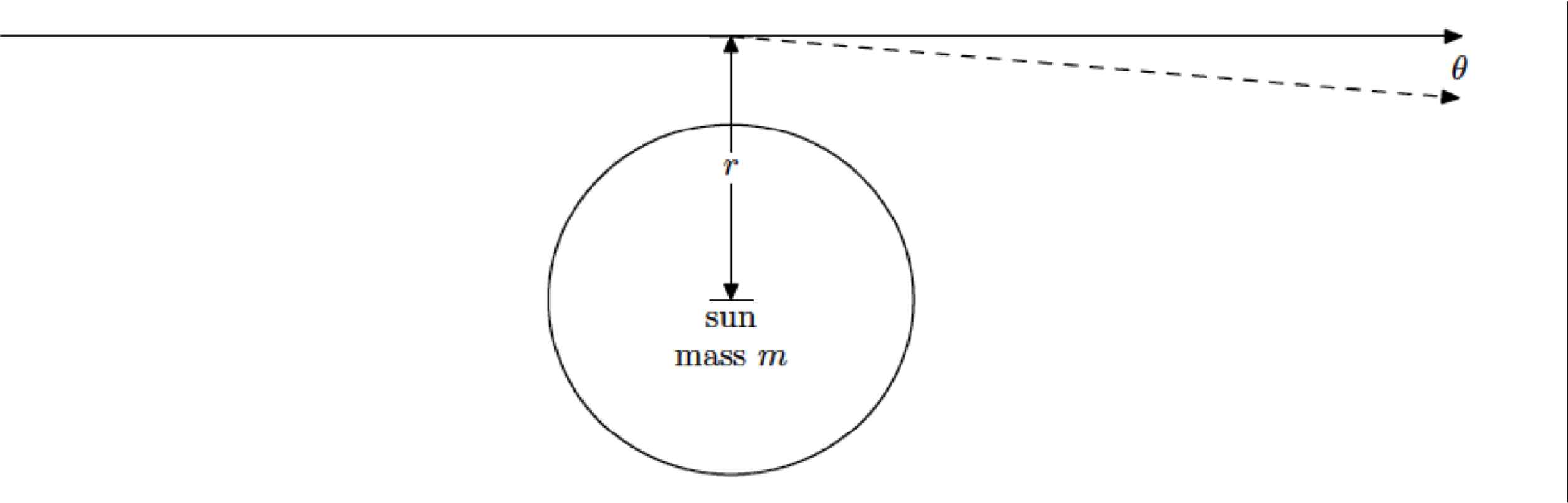
Schematic light deflection by the sun.
The associated fractional energy change
We have no idea about the proportionality factor, the classical mechanics yields 2, GR requires the solution of the geodesic equations, not exactly an easy task [19–22]. The conclusion of the computation is a factor 4.
It is evident that the deflection is proportional to mass; in our solar system the largest mass is the sun, using therefore the relevant parameters we find θ ≅ 2 · 10−6 rad. The experiment [20] measured 8 · 10−6 rad in agreement with the Einstein prediction.
The gravitational redshift [19–21], namely the phenomenon of loose of energy of a photon moving through a gravitational field, is a naïve consequence of the previous discussion. We have indeed
Even though not immediately recognized, the previous relations have close relevance to the problem of Mercury perihelion precession, which owing to its closer proximity to the sun is more significantly affected by GR corrections. This means that a massive object modifies either the spatial and time structure of the space time metric
The change of metrics determines a change in the GR Kepler equation, which determines an emerging new term correcting the Newtonian result [20–23]. According to this correction, the revolution angle around the sun executed in one year by the planet is [19–23]
The advance per year of the perihelion can be seen in Fig. 4.
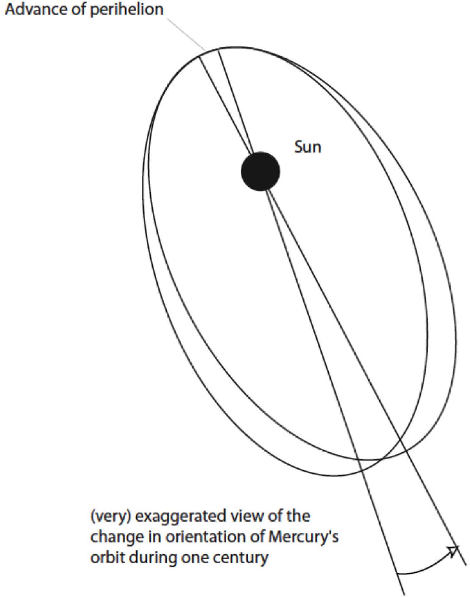
Mercury perihelion precession.
These tiny effects, ruled by the dimensionless constant
This means that the absolute error accumulated in one day (86,400s) is ∆T ≅ 4.3 · 10−5 s, and the associated error (if not corrected) in measuring length (∆L = c∆T) would be about 14 km [19].
Before closing this topic, we like to mention the “heterodox” speculations recently published [24] in which GR predictions, like Mercury perihelion precession, have been ascribed to a structure of the space time viewed as a “dilatant-fluid” which, among other things, produces a kind of viscosity determining the deceleration of spaceships during their motion. The speculations in [24] have been motivated by the so-called Pioneer anomaly [25], consisting in a much shorter traveled distance with respect to that predicted by the computation. The deceleration inferred from the trajectory data has been estimated to be −8.74 · 10−10 m · s−2, a value which has been justified including in the equations of motion the effect of the recoil of the photons emitted via black-body radiation by the spacecraft. The alternative explanation put forward in [26] is that of assuming a drag force which has some resemblance with the already quoted Stokes force including the viscosity. As it is well known the Stokes force is written as
Putting this force in the classical equation for the planet motion and replacing the orbital velocity with
The results in Eq. (106) are equivalent to those in Eq. (99) and have been obtained within the context of classical mechanics, with special relativity corrections included in the dilatant part of the Stokes term. In both formulations the leading corrections are due to the dimensionless parameter GM/(Rc2).
Why have we reported this example?
Not to deny the GR to give credit to the (doubtful) introduction of an ad hoc force causing decelerating effects, rather to corroborate the importance of non-dimensional parameters which, once properly chosen, may provide a useful hint even though inserted in not a properly rigorous physical and mathematical context (see also our previous derivations of gravitational redshift and light deflection).
5.2. Quantum Mechanics and Dimensional Analysis
We have tried to convey the importance of thinking in terms of dimensions and what may be the impact on different aspects of Physical discipline. We must add a warning, which is absolutely necessary to be extremely cautious in using the tool we have described. The use of DA requires experience to guess an appropriate list of physical quantities. The wrong list would lead to meaningless results. An example, in absence of the Planck constant, the attempt of determining the size of atoms resulted in a complete failure [27,28].
The idea of introducing Planck’s constant as a fundamental quantity in atomic physics was disregarded for some time (a decade since the Planck paper on Black-Body radiation [29]). It had not yet the status of a fundamental constant, it being associated with thermal phenomena. It was, as noted in [28], a constant to be explained rather than to be used for explanations. It was later shown that charge mass and h can be combined to get a length (see below) but this observation did not provide any further progress, since nobody had indicated how the combination of this quantity had to come in the analysis of atomic structure.
The breakthrough came with the Bohr paper [30] and this is well known, but there were earlier suggestions and this story is worth to be mentioned. To the authors’ knowledge the first towards the search for a connection between the quantum of action and the atoms was Haas in his study of the stability of Thomson’s atom [31].
The reasoning of Haas was as follows. His main assumption was that one electron on the surface of an atom is attracted by the +Ne charge of the nucleus and repelled by the other remaining (N–1) electrons. If the charges are symmetrically distributed the electrons would experience the attraction of a single positive charge. If the centrifugal force is compared to the Coulomb attractive force one can get the speed of the electron around the nucleus, namely
The electron rotation period around the nucleus is therefore
The next and final step by Haas was the assumption that the electron potential energy multiplied by the revolution time is just the Planck constant ħ (a quantity with the dimensions of an action, see below) namely
However, the intent of Haas was that of specifying the Planck constant (the mysterious quantity at the time) in terms of the atom parameters instead of the contrary. This attempt by Haas was not taken in due consideration and was strongly criticized for mixing up thermodynamics and mechanics. The importance of the idea was later recognized.
We can now proceed in terms of DA and see how the problem should be correctly afforded. The atomic size is dominated by forces of electromagnetic nature, we list accordingly physical quantities, r (Atomic Radius), h (Planck constant), ɛ0 (electric permittivity), me (electron mass) and e (electron charge). We are now obliged to enlarge our system of fundamental units, by including the charge whose dimensions are denoted by [Q]. We can therefore set
Recalling that h has the dimensions of an action [ET] and [ε0] = [Q2F−1L−2], we have five physical quantities and four repeating variables and therefore we end up with (κ is a constant)
Which introducing the fine structure constant
We have mentioned the constant α, a number which has created a great deal of speculation in the past. An account of this debate is outside of the scope of this paper; the interested reader is therefore referred to [32] where a survey is presented.
A final example we want to discuss is the derivation of the physical dimension of the magnetic charges (assuming that they exist) [33].
We remind that the force acting on electric and magnetic charges at rest in SI units are (μ0 is the vacuum magnetic permeability)
Multiplying both sides of the previous equations, we get
Recalling that
Noting furthermore that [EH] has the same dimensions of the Poynting vector, namely Power/Surface, we end up with
From the dimensional point of view the product of an electric and a magnetic charge is an angular momentum. This would open further speculations on Dirac monopoles and charge quantization [33], which in unit of the reduced Planck constant can be written as
The relevant technical details go well beyond the scope of this article and will not be included in the present discussion.
6. FINAL COMMENTS
In this paper, we have put together different examples from diverse branches of Physics. There are problems which we did not even touch, for example, regarding the nondimensionalization of differential equations describing a physical phenomenon.
The Navier-Stokes equation accounts for the momentum conservation of an incompressible fluid. It can be cast in the form
The procedure of nondimensionalization has revealed two other quantities of crucial importance in the dynamics of fluids, namely the Stroudhal [34] and Euler [35] numbers.
Without entering into a discussion of the relevant importance, we note that the second represents the ratio between pressure and kinetic pressure. It is related to the cavitation number, which quantifies the potential of a flow to cavitate, namely the ability of a fluid to create bubbles, which after collapsing create a shock wave damaging machineries of a ship.
The Stroudhal number is important whenever non-stationary (oscillating) fluids are considered. It represents indeed a measure of the ratio of the inertial forces to those associated with the unsteadiness of the flow. If it turns out to be a small quantity with respect to the others entering the normalized form of the Navier-Stokes equation, the problem can be considered stationary.
Before concluding, we like to go back the incipit of the article where we have mentioned the concept of dimension in Euclidean geometry, in which we have defined dimensions of integer order (0, 1, 2, 3). The Fractal geometry admits non-integer dimensions. This has opened new avenues in the understanding of the interplay between (physical/geometrical) dimensions and scaling laws. This aspect of the problem will be the topic of a forthcoming investigation.
We hope that we have provided at least two feelings:
- •
The problem of physical dimensions is an issue of fundamental importance in Physics, rich of conceptual aspects and providing unsuspected links between apparently uncorrelated fields.
- •
Our paper, albeit long, has scratched the surface of a huge field of research.
Regarding this last point, we have ignored important aspects of the discussion like those associated with the renormalization group, DA in quantum field theory and dimensional collapse. These topics deserve a deeper understanding of the problems and are worth to be treated in a separate discussion.
Footnotes
U instead of V to avoid confusion with volume.
We remind that the theorem asserts that the variation of the kinetic energy of a body is equivalent to the work done on that body.
This choice is just matter of convenience.
The differential form of the Gauss’s law for gravity assumes the expression ∇2ϕ = 4πGρ, being ϕ a scalar potential.
The MOL in the SI denotes the unit measuring the amount of a substance.
REFERENCES
Cite This Article
TY  - JOUR
AU  - G. Dattoli
AU  - E. Di Palma
AU  - E. Sabia
PY  - 2022
DA  - 2022/05/06
TI  - Is There Anything Interesting to Say About Dimensions in Physics?
JO  - Growth and Form
SP  - 3
EP  - 25
VL  - 3
IS  - 1-2
SN  - 2589-8426
UR  - https://doi.org/10.55060/j.gandf.220605.001
DO  - https://doi.org/10.55060/j.gandf.220605.001
ID  - Dattoli2022
ER  -


